Chapter 5 Continuous Distributions

5.1 Probability Density Function (pdf)

Probability density function is used to describe a continuous distribution.

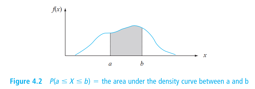
Let \(X\) be a continuous rv. Then a probability density function (pdf) of \(X\) is a function \(f(x)\) such that for any two numbers \(a\) and \(b\) with \(a \le b\), \[ P(a\le X\le b)=\int_a^b f(x)dx \] That is, the probability that \(X\) takes on a value in the interval \([a, b]\) is the area above this interval and under the graph of the density function. The graph of \(f(x)\) is often referred to as the density curve.

For \(f(x)\) to be a legitimate pdf, it must satisfy the following two conditions:

• \(f(x)\ge 0\) for all \(x\)
• \(\int_{-\infty}^\infty f(x)dx=\text{area under the entire curve of }f(x)=1\).

5.2 Cumulative Distribution Function (cdf)

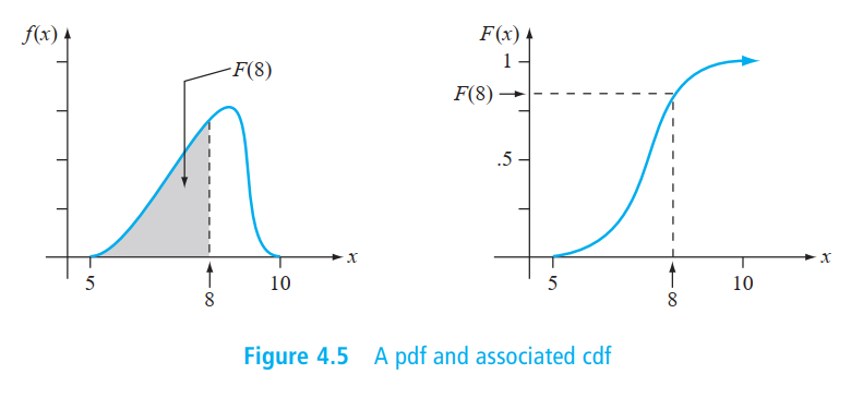
The cumulative distribution function F(x) for a continuous rv \(X\) is defined for every number \(x\) by
\[ F(x)=P(X\le x)=\int_{-\infty}^x f(y)dy. \] For each \(x\), \(F(x)\) is the area under the density curve to the left of \(x\).

Using \(F(x)\) to Compute Probabilities:

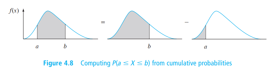
Let \(X\) be a continuous rv with pdf \(f(x)\) and cdf \(F(x)\). Then for any number \(a\), \[ P(X>a)=1-F(a) \] and for any two numbers \(a\) and \(b\) with \(a<b\), \[ P(a\le X\le b)=F(b)-F(a). \]

Obtaining \(f(x)\) from \(F(x)\):

If \(X\) is a continuous rv with pdf \(f(x)\) and cdf \(F(x)\), then at every \(x\) at which the derivative \(F'(x)\) exists, \(F'(x)=f(x)\).

5.3 Expected Values and Variance

The expected or mean value of a continuous rv \(X\) with pdf \(f(x)\) is
\[ \mu_X=E(X)=\int_{-\infty}^\infty x\cdot f(x)dx. \] If \(X\) is a continuous rv with pdf \(f(x)\) and \(h(X)\) is any function of \(X\), then
\[ E[h(X)]=\mu_{h(X)}=\int_{-\infty}^\infty h(x)\cdot f(x)dx. \] The variance of a continuous random variable \(X\) with pdf \(f(x)\) and mean value \(\mu\) is \[ \sigma^2_X=V(X)=\int_{-\infty}^\infty(x-\mu)^2\cdot f(x)dx. \] The standard deviation (SD) of \(X\) is \(\sigma_X=\sqrt{V(X)}\).

Shortcut formula to compute variance: \[ V(X)=E(X^2)-[E(X)]^2. \]

5.4 Uniform Distribution

A continuous rv \(X\) is said to have a uniform distribution on the interval \([A, B]\) if the pdf of X is
\[ f(x; A, B)=\left\{ \begin{array}{rc} \frac{1}{B-A} & A\le x\le B \\ 0 & \text{otherwise} \end{array}\right. \] Uniform distribution is called “uniform” because its probability density is identical everywhere.

5.5 Normal Distribution

A continuous rv \(X\) is said to have a normal distribution with parameters \(\mu\) and \(\sigma\) (or \(\mu\) and \(\sigma^2\)), where \(-\infty<\mu<\infty\) and \(\sigma>0\), if the pdf of \(X\) is \[ f(x;\mu,\sigma)=\frac{1}{\sqrt{2\pi\sigma^2}}\exp\left[-\frac{1}{2}\left(\frac{x-\mu}{\sigma}\right)^2\right], \;\;\;-\infty<x<\infty. \]

Standard normal distribution

The normal distribution with parameter values \(\mu=0\) and \(\sigma=1\)​ is called the standard normal distribution. A random variable having a standard normal distribution is called a standard normal random variable and will be denoted by \(Z\). The pdf of \(Z\) is \[ f(x;0,1)=\frac{1}{\sqrt{2\pi}}\exp\left(-\frac{z^2}{2}\right), \;\;\;-\infty<x<\infty. \] If \(X\) has normal distribution with parameters \(\mu\) and \(\sigma\), then \[ \frac{X-\mu}{\sigma} \] has the standard normal distribution. The process of \((X-\mu)/\sigma\) is called standardization.

The standard normal distribution is mainly used to compute the probability in non-standard normal distributions, \[ \begin{split} P(a\le X\le b)&=P\left(\frac{a-\mu}{\sigma}\le \frac{X-\mu}{\sigma}\le \frac{b-\mu}{\sigma}\right) \\ &=P\left(\frac{a-\mu}{\sigma}\le Z \le \frac{b-\mu}{\sigma}\right) \\ &=\Phi\left(\frac{b-\mu}{\sigma}\right)-\Phi\left(\frac{a-\mu}{\sigma}\right), \end{split} \]

\[ P(X\le a)=\Phi\left(\frac{a-\mu}{\sigma}\right) \]

\[ P(X\ge b)=1-\Phi\left(\frac{b-\mu}{\sigma}\right) \]

where \(\Phi\) is the cdf of standard normal distribution.

If the population distribution of a variable is (approximately) normal, then

• Roughly \(68\%\) of the values are within \(1\) SD of the mean.

• Roughly \(95\%\) of the values are within \(2\) SDs of the mean.

• Roughly \(99.7\%\) of the values are within \(3\) SDs of the mean.

Normal approximation of binomial distribution

Let \(X\) be a binomial rv based on \(n\) trials with success probability \(p\). Then if the binomial probability histogram is not too skewed, \(X\) has approximately a normal distribution with \(\mu=np\) and \(\sigma=\sqrt{np(1-p)}\). In particular, for \(x=\) a possible value of \(X\),
\[ P(X\le x) \approx \Phi\left(\frac{x+.5-np}{\sqrt{np(1-p)}}\right) \] In practice, the approximation is adequate provided that both \(np\ge 10\) and \(n(1-p)\ge 10\) , since there is then enough symmetry in the underlying binomial distribution.

5.6 Exponential Distribution

Recall of Poisson distribution:

In a situation, the probability of a single event occurring is proportional to the waiting time. For example, the event is that a bus arriving at a bus station, a customer arriving at a store, a call into a calling center.

The average number of occurrent during per unit of time (such as per minute, per hour) is called “RATE”. An example of rate can be the average number of bus arriving at a bus station in an hour. We often denote the rate with the Greek letter λ.

A rv \(X\) is said to have an exponential distribution with rate parameter \(\lambda\) if the pdf of \(X\) is
\[ f(x; \lambda)=\left\{ \begin{array}{rc} \lambda e^{-\lambda x} & x\ge 0 \\ 0 & \text{otherwise} \end{array}\right. \] Exponential distribution is used to describe the waiting time between two occurrence of Poisson events. It can be the waiting time to the first occurrence or the waiting time between any two adjacent occurrence.

5.7 Gamma Distribution

Gamma function

For \(\alpha>0\), the gamma function \(\Gamma(\alpha)\) is defined by \[ \Gamma(\alpha)=\int_0^\infty x^{\alpha-1}e^{-x}dx. \] Properties of gamma functions:

• For any \(\alpha>1\), \(\Gamma(\alpha)=(\alpha-1)\cdot\Gamma(\alpha-1)\);
• For any positive integer \(n\), \(\Gamma(n)=(n-1)!\);
• \(\Gamma(1/2)=\sqrt \pi\).

A continuous random variable \(X\) is said to have a gamma distribution if the pdf of \(X\) is
\[ f(x; \alpha,\beta)=\left\{ \begin{array}{rc} \frac{1}{\beta^\alpha\Gamma(\alpha)}x^{\alpha-1}e^{-x/\beta} & x\ge 0 \\ 0 & \text{otherwise} \end{array}\right. \] where the parameter \(\alpha\) is called the shape parameter and \(\beta\) is called the scale parameter. The standard gamma distribution has \(\beta=1\).

Alternatively, the pdf of a gamma distribution can be written as \[ f(x; \alpha,\lambda)=\left\{ \begin{array}{rc} \frac{\lambda^\alpha}{\Gamma(\alpha)}x^{\alpha-1}e^{-\lambda x} & x\ge 0 \\ 0 & \text{otherwise} \end{array}\right. \] where the RATE parameter \(\lambda\) is equal to \(1/\beta\).

A gamma distribution is typically used to describe the waiting time till the \(\alpha\)th occurrence of Poisson event when the shape parameter \(\alpha\) is integer.

5.8 Chi-squared Distribution

Let \(a\) be positive integer. Then a random variable \(X\) is said to have a chis-quared distribution with parameter if the pdf of \(X\) is the gamma density with \(\alpha=\nu/2\) and \(\beta=2\). The pdf of a chi-squared rv is thus
\[ f(x; \alpha,\beta)=\left\{ \begin{array}{rc} \frac{1}{2^{\nu/2}\Gamma(\nu/2)}x^{\frac{\nu}{2}-1}e^{-\frac{x}{2}} & x\ge 0 \\ 0 & \text{otherwise} \end{array}\right. \] The parameter \(\nu\) is called the degrees of freedom (df). The symbol \(\chi^2\) is often used in place of “chi-squared”.

The chi-squared distribution is often used to describe the distribution of the sum of \(\nu\) independent standard normal rvs.

5.9 Relationship between Poisson, Exponential and Gamma Distributions

5.9.1 Postulates of Poisson Process

1. The probability that at least one Poisson arrival occurs in a small time period Δt is “approximately” λΔt. Here λ is called the arrival-rate parameter of the process.
2. The number of Poisson-type arrivals happening in any prespecified time interval of fixed length is not dependent on the “starting time” of the interval or on the total number of Poisson arrivals recorded prior to the interval.
3. The numbers of arrivals happening in disjoint time intervals are mutually independent random variables.
4. Given that one Poisson arrival occurs at a particular time, the conditional probability that another occurs at exactly the same time is zero.

Once an experiment satisfy all these four assumptions, it is a Poisson process. From the Poisson process, we can derive three distributions:

• Poisson distribution (about the number of occurrence during a fix time interval \(t\))
• Exponential distribution (about the waiting time between two subsequent occurrence)
• Gamma distributions (about the waiting time before the \(\alpha\)th occurrence)

5.10 Beta Distribution

A random variable \(X\) is said to have a beta distribution with parameters (both positive), \(A\), and \(B\) if the pdf of \(X\)​ is
\[ f(x; \alpha,\beta, A, B)=\left\{ \begin{array}{rc} \frac{1}{B-A}\cdot \frac{\Gamma(\alpha+\beta)}{\Gamma(\alpha)\Gamma(\beta)} \left(\frac{x-A}{B-A}\right)^{\alpha-1} \left(\frac{B-x}{B-A}\right)^{\beta-1} & A\le x\le B \\ 0 & \text{otherwise} \end{array}\right. \] The case \(A=0\), \(B=1\) gives the standard beta distribution.

The standard beta distribution has pdf \[ f(x; \alpha,\beta)=\left\{ \begin{array}{rc} \frac{x^{\alpha-1}(1-x)^{\beta-1}}{B(\alpha,\beta)} & 0\le x\le 1 \\ 0 & \text{otherwise} \end{array}\right. \] where \(B(\alpha,\beta)=\frac{\Gamma(\alpha)\Gamma(\beta)}{\Gamma(\alpha+\beta)}\) is called Beta function.

The standard Beta distribution is “a distribution of Bernoulli distributions”. We can create a “random” Bernoulli distribution by drawing a probability \(p\sim Beta(\alpha, \beta)\).