Chapter 6 Joint Distributions and Correlation
6.1 Two Discrete rv
The probability mass function (pmf) of a single discrete rv \(X\) specifies how much probability mass is placed on each possible \(X\) value. The joint pmf of two discrete rv’s \(X\) and \(Y\) describes how much probability mass is placed on each possible pair of values \((x, y)\).
Let \(X\) and \(Y\) be two discrete rv’s defined on the sample space of an experiment. The joint probability mass function \(p(x, y)\) is defined for each pair of numbers \((x, y)\) by \[ p(x, y)=P(X=x \text{ and } Y=y). \] It must be the case that \(p(x, y)\ge 0\) and \(\underset{x}{\sum}\underset{y}{\sum} p(x, y)=1\).
Now let \(A\) be any set consisting of pairs of \((x, y)\) values (e.g., \(A = \{(x, y): x +y= 5 \}\) or \(A = \{(x, y): max(x,y)\le3 \}\). Then the probability \(P\left[(X, Y) \in A\right]\) is obtained by summing the joint pmf over pairs in \(A\): \[ P\left[(X, Y) \in A\right]=\underset{(x,y)\in A}{\sum\sum}p(x, y) \]
For example, given joint pmf of \(X\) and \(Y\) in Figure 6.1,
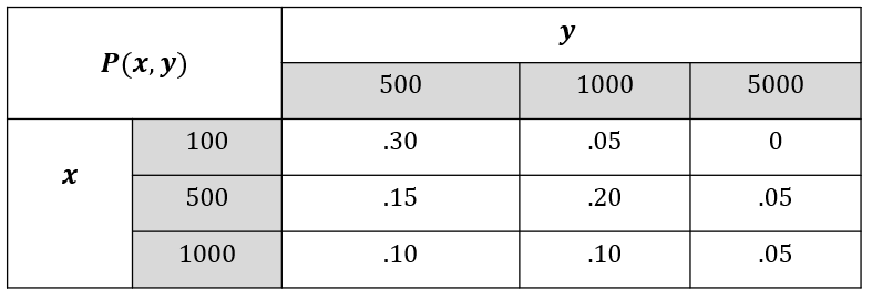
Figure 6.1: Joint pmf.
Figure 6.2: Event of X=Y.
Figure 6.3: Event of X greater or equal to Y.
6.2 Marginal Distribution
The marginal probability mass function of \(X\), denoted by \(p_X(x)\), is given by
\[
p_X(x)=\underset{y}{\sum}p(x,y) \;\text{ for each possible value }x
\]
Similarly, the marginal probability mass function of \(Y\) is
\[
p_X(x)=\underset{x}{\sum}p(x,y) \;\text{ for each possible value }y
\]
The use of the word “marginal” here is a consequence of the fact that if the joint pmf is displayed in a rectangular table, then the row totals give the marginal pmf of \(X\) and the column totals give the marginal pmf of \(Y\), as is seen in Figure 6.4.
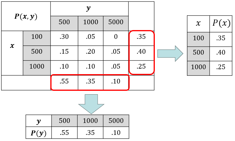
Figure 6.4: Marginal pmfs.
6.3 Two Continuous rv
Let \(X\) and \(Y\) be continuous rv’s. A joint probability density function \(f(x, y)\) for these two variables is a function satisfying \(f(x, y)\ge 0\) and \(\int_{-\infty}^\infty\int_{-\infty}^\infty f(x,y)dxdy=1\). Then for any two-dimensional set \(A\) \[ P\left[(X,Y)\in A\right]=\underset{A}{\int\int} f(x,y)dxdy \] In particular, if \(A\) is the two-dimensional rectangle \(\{(x, y): a \le x \le b, c \le y \le d\}\).
We can think of \(f(x, y)\) as specifying a surface at height \(f(x, y)\) above the point \((x, y)\) in a three-dimensional coordinate system. Then \(P[(X, Y) \in A]\) is the volume underneath this surface and above the region \(A\), analogous to the area under a curve in the case of a single rv.

Example
A bank operates both a drive-up facility and a walk-up window. On a randomly selected day, let \(X=\) the proportion of time that the drive-up facility is in use (at least one customer is being served or waiting to be served) and \(Y=\) the proportion of time that the walk-up window is in use. Then the set of possible values for \((X, Y)\) is the rectangle \(D = \{(x, y): 0 \le x \le 1, 0 \le y \le 1\}\). Suppose the joint pdf of \((X, Y)\) is given by
\[
f(x,y) = \left\{ \begin{array}{rc}
\frac{6}{5}(x+y^2) & 0\le x\le 1,\; 0\le y\le 1
\\
0 & \text{otherwise}
\end{array}\right.
\]
To verify that this is a legitimate pdf, note that \(f(x, y) \ge 0\) and
\[
\begin{split}
\int_{-\infty}^\infty\int_{-\infty}^\infty f(x,y)dxdy&=\int_0^1\int_0^1 \frac{6}{5}(x+y^2) dxdy
\\
&=\int_0^1\int_0^1 \frac{6}{5}xdxdy+\int_0^1\int_0^1 \frac{6}{5}y^2dxdy
\\
&=\int_0^1\frac{6}{5}xdx+\int_0^1 \frac{6}{5}y^2dy
\\
&=\frac{6}{10}+\frac{6}{15}=1
\end{split}
\]
The probability that neither facility is busy more than one-quarter of the time is
\[
\begin{split}
P\left( 0 \le X \le \frac{1}{4}, 0 \le Y \le \frac{1}{4} \right)&=\int_0^{1/4}\int_0^{1/4} \frac{6}{5}(x+y^2) dxdy
\\
&=\int_0^{1/4}\int_0^{1/4} \frac{6}{5}xdxdy+\int_0^{1/4}\int_0^{1/4} \frac{6}{5}y^2dxdy
\\
&=\frac{6}{20}\cdot\frac{x^2}{2}\bigg|_{x=0}^{x=1/4}+\frac{6}{20}\cdot\frac{y^3}{3}\bigg|_{y=0}^{y=1/4}
\\
&=\frac{7}{640}=.0109
\end{split}
\]
The marginal pdf of each variable can be obtained in a manner analogous to what we did in the case of two discrete variables. The marginal pdf of \(X\) at the value \(x\) results from holding \(x\) fixed in the pair \((x, y)\) and integrating the joint pdf over \(y\). Integrating the joint pdf with respect to \(x\) gives the marginal pdf of \(Y\).
The marginal probability density functions of \(X\) and \(Y\), denoted by \(f_X(x)\) and \(f_Y(y)\), respectively, are given by
\[
f_X(x)=\int_{-\infty}^\infty f(x,y)dy \;\;\;\;\;\; \text{for } -\infty \le x \le \infty
\]
\[ f_Y(y)=\int_{-\infty}^\infty f(x,y)dx \;\;\;\;\;\; \text{for } -\infty \le y \le \infty \]
In the previous example, the marginal pdf of \(X\), which gives the probability distribution of busy time for the drive-up facility without reference to the walk-up window, is
\[
f_X(x)=\int_{-\infty}^\infty f(x,y)dy=\int_0^1 \frac{6}{5}(x+y^2)dy=\frac{6}{5}x+\frac{2}{5}
\]
for \(0\le x\le 1\) amd \(0\) otherwise. The marginal pdf of \(Y\) is
\[
f_Y(x) = \left\{ \begin{array}{rc}
\frac{6}{5}y^2+\frac{3}{5} & 0\le y\le 1
\\
0 & \text{otherwise}
\end{array}\right.
\]
Then
\[
P\left( \frac{1}{4}\le Y\le\frac{3}{4}\right)=\int_{1/4}^{3/4} f_Y(y)dy=\frac{37}{80}=.4625
\]
6.4 Independence
Two random variables \(X\) and \(Y\) are said to be independent if for every pair of \(x\) and \(y\) values \[ p(x, y)=p_X(x)\cdot p_Y(y)\;\;\;\;\;\;\text{when $X$ and $Y$ are discrete} \] or \[ f(x, y)=f_X(x)\cdot f_Y(y)\;\;\;\;\;\;\text{when $X$ and $Y$ are continuous} \] Otherwise, they are dependent.
Example
in Figure 6.4, \(p(1000, 5000)=.05 \ne p(X=1000)\times p(Y=5000)=.25\times.1\), thus, \(X\) and \(Y\) are NOT independent.
6.5 Conditional Distributions
Suppose \(X =\) the number of major defects in a randomly selected new car and \(Y =\) the number of minor defects in that same car. If we learn that the selected car has one major defect, what now is the probability that the car has at most three minor defects — that is, what is \(P(Y \le 3 | X = 1)\)?
Questions of this sort can be answered by studying conditional probability distributions.
Let \(X\) and \(Y\) be two continuous rv’s with joint pdf \(f(x, y)\) and marginal \(X\) pdf \(f_X(x)\). Then for any X value \(x\) for which \(f_X(x)>0\), the conditional probability density function of \(Y\) given that \(X=x\) is
\[
f_{Y\mid X}(y\mid x)=\frac{f(x, y)}{f_X(x)}\;\;\;\;\;\; -\infty < y<\infty
\]
If \(X\) and \(Y\) are discrete, replacing pdfs by pmfs in this definition gives the conditional probability mass function of \(Y\) when \(X=x\).
Example 5.12
Reconsider the situation of Examples 5.3 and 5.4 involving \(X=\) the proportion of time that a bank’s drive-up facility is busy and \(Y=\) the analogous proportion for the walk-up window. The conditional pdf of \(Y\) given that \(X=.8\) is
\[
f_{Y\mid X}(y\mid x)=\frac{f(.8, y)}{f_X(.8)}=\frac{1.2(.8+y^2)}{1.2(.8)+.4}=\frac{1}{34}(24+30y^2) \;\;\;0 < y<1
\]
The probability that the walk-up facility is busy at most half the time given that \(X=.8\) is then
\[
P(Y\le.5 \mid X=.8)=\int_{-\infty}^.5 f_{Y\mid X}(y\mid.8)dy=\int_0^5 \frac{1}{34}(24+30y^2)dy=.390
\]
Using the marginal pdf of \(Y\) gives \(P(Y \le .5) =5 =.350\). Also \(E(Y) = .6\), whereas the expected proportion of time that the walk-up facility is busy given that \(X = .8\) (a conditional expectation) is
\[
E(Y\mid X=.8)=\int_{-\infty}^\infty y\cdot f_{Y\mid X}(y\mid .8)dy=\frac{1}{34}\int_0^1 y(24+30y^2) dy=.574
\]
If the two variables are independent, the marginal pmf or pdf in the denominator will cancel the corresponding factor in the numerator. The conditional distribution is then identical to the corresponding marginal distribution.
6.6 Expected Values
Let X and Y be jointly distributed rv’s with pmf p(x, y) or pdf f(x, y) accordingto whether the variables are discrete or continuous. Then the expected value of a function h(X, Y), denoted by E[h(X, Y)] or mh(X, Y), is given by \[ E\left[h(x,y)\right]= \left\{ \begin{array}{ll} \underset{x}{\sum}\underset{y}{\sum} h(x,y)\cdot p(x, y) & \text{if X and Y are discrete} \\ \int_{-\infty}^\infty\int_{-\infty}^\infty h(x,y)\cdot f(x, y)dxdy & \text{if X and Y are continous} \end{array}\right. \]
Example 5.13
Five friends have purchased tickets to a certain concert. If the tickets are for seats 1–5 in a particular row and the tickets are randomly distributed among the five, what is the expected number of seats separating any particular two of the five? Let X and Y denote the seat numbers of the first and second individuals, respectively. Possible \((X, Y)\) pairs are \(\{(1, 2), (1, 3), \cdots , (5, 4)\}\), and the joint pmf of \((X, Y)\) is
\[
p(x,y) = \left\{ \begin{array}{rc}
\frac{1}{20} & x=1,\ldots, 5;\; x=1,\ldots, 5;x\ne y
\\
0 & \text{otherwise}
\end{array}\right.
\]
The number of seats separating the two individuals is \(h(X, Y) = |X - Y | - 1\). The accompanying table gives \(h(x, y)\) for each possible \((x, y)\) pair.

Thus, \[ E(h(X, Y))=\underset{(x, y)}{\sum\sum} h(x, y)\cdot p(x, y)=\underset{x\ne y}{\sum_{x=1}^5\sum_{x=1}^5} (|X - Y|-1)\cdot \cdot \frac{1}{20}=1 \]
6.7 Covariance
Covariance is used to measure the linear dependence between two random variables.
The covariance between two rv’s \(X\) and \(Y\) is \[ \begin{split} Cov(X, Y)&=E\left[(X-\mu_X)(Y-\mu_Y)\right] \\ \\ &= \left\{ \begin{array}{ll} \underset{x}{\sum}\underset{y}{\sum} (x-\mu_X)(y-\mu_Y)\cdot p(x, y) & \text{if X and Y are discrete} \\ \int_{-\infty}^\infty\int_{-\infty}^\infty (x-\mu_X)(y-\mu_Y)\cdot f(x, y)dxdy & \text{if X and Y are continous} \end{array}\right. \end{split} \] Shortcut formula \[ Cov(X, Y)=E(XY)-\mu_X\cdot\mu_Y \]
Property of covariance: \[ Cov(aX+b, cY+d)=ab\cdot Cov(X, Y) \] This property tells us that the covariance between two rvs will change after linear transformations (\(Cov\) is NOT invariant to linear transformation).
We all know height and weight are correlated. If we use covariance as the measure of dependence, what problems will happen? The covariance will change when we switch from Imperial system to Metric!
6.8 Correlation
Correlation is the standardized covariance, and it is invariant to linear transformation.
The correlation coefficient of \(X\) and \(Y\), denoted by \(Corr(X, Y)\), \(\rho_{X,Y}\), or just \(\rho\), is defined by
\[
\rho_{X,Y}=\frac{Cov(X, Y)}{\sigma_X\cdot \sigma_Y}
\]
Properties:
If a and c are either both positive or both negative,
\[ Corr(aX + b, cY + d) = Corr(X, Y). \] In other words, a linear transformation does not change the correlation.For any two rv’s \(X\) and \(Y\), \(-1 \le Corr(X, Y) \le 1\).
If \(X\) and \(Y\) are independent, then \(\rho=0\), but \(\rho=0\) does not imply independence.
\(\rho=1\) or \(-1\) if and only if \(Y=aX+b\) for some numbers \(a\) and \(b\) with \(a\ne 0\).