Chapter 2 Set Theory and Probabilities

2.1 Terminologies

Chance experiment is any activity or process whose outcome is subject to uncertainty. The simplest experiment to which probability applies is one with two possible outcomes, such as flipping a coin.
Sample space, denoted as $\mathcal S$, the collection of all possible outcomes of a chance experiment.
An event is any collection of outcomes (subset) from the sample space of a chance experiment.

2.2 Types of Events

If an event consists of exactly one outcome, we call it simple event/elementary event;
If an event consists of more than one outcome, we call it compound event;
If an event consists of no outcome, we call it null event, denoted as $\varnothing$.

2.3 Relationships between Events

The complement of an event $A$, denoted as $A^c$ or $A'$, is the set of all outcomes in $\mathcal S$ that are not contained in $A$;

Figure 2.1: Venn diagram of Complement.

The union of two events $A$ and $B$, denoted by $A \cup B$ and read “$A$ or $B$”, is the event consisting of all outcomes that are either in A or in B or in both events. That is, all outcomes in at least one of the events.

Beware that the union includes outcomes for which both A and B occur as well as outcomes for which exactly one occur.

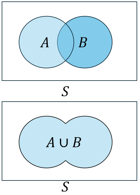
Figure 2.2: Venn diagram of Union.

The intersection of two events $A$ and $B$, denoted by $A \cap B$ and read “$A$ and $B$”, is the event consisting of all outcomes that are in both $A$ and $B$.

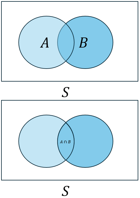
Figure 2.3: Venn diagram of the intersection of A and B.

Let $\varnothing$ denote the null event (the event consisting of no outcomes). When $A \cap B=\varnothing$, $A$ and $B$ are mutually exclusive or disjoint events.

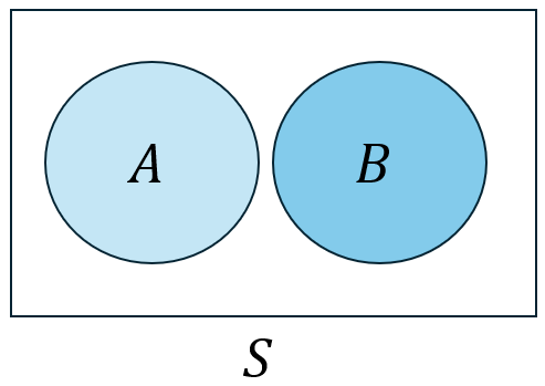
Figure 2.4: Venn diagram of two mutually exclusive/disjoint events.

2.4 Algebra of Events

The operation of forming unions, intersections, and the complements of events obey certain rules:

Commutative law \[ A \cup B=B\cup A, \\ A \cap B=B\cap A; \]
Associate law \[ (A\cup B)\cup C = A \cup (B\cup C), \\ (A \cap B)\cap C = A \cap (B\cap C); \]
Distributive law \[ (A\cup B) \cap C= (A \cap C) \cup (B \cap C) \\ (A\cap B) \cup C= (A \cup C) \cap (B \cup C) \]
De Morgan’s law \[ (A \cup B)^c=A^c \cap B^c \\ (A \cap B)^c=A^c \cup B^c \]

2.5 Axioms of Probabilities

Axiom 1 (Non-negativity): For any event A, $P(A) \ge 0$.

Axiom 2 (Normativity): $P(\mathcal S)=1$.

Recall: Sample space itself is also an event, which has probability equal to one.

Axiom 3 (Countable additivity): If $A_1, A_2, A_3, \ldots$ is an infinite collection of disjoint events, then \[ P(A_1 \cup A_2 \cup A_3 \cup \cdots)=\sum_{i=1}^\infty P(A_i). \]

The axioms serve to rule out probability assignments that are inconsistent with our intuition.

2.6 Properties of Probabilities

These propositions are derived from three axioms of probabilities.

Proposition 1: $P(\varnothing)=0$, where $$ is the null event (the event containing no outcomes whatsoever). This in turn implies that the property contained in Axiom 3 is valid for a finite collection of disjoint events.

\[ P(A_1\cup A_2 \cup A_3 \cup \cdots A_n) = \sum_{i=1}^n P(A_i). \]

Proposition 2: For any event $A$ and its complement event $A^c$, \[ P(A)=1-P(A^c). \]

This proposition is surprisingly useful because there are many situations in which $P(A^c)$ is more easily obtained by direct methods than is P(A).

Proposition 3: For any event $A$, \[ P(A)\le 1 . \]

Proposition 4 (Addition Rule): For any two events A and B, \[ P (A\cup B)=P(A)+P(B)-P(A\cap B) \]

For any three events A, B and C, \[ P (A\cup B \cup C)=P(A)+P(B)+P(C)-P(A\cap B)-P(A\cap C)-P(B\cap C)+P(A \cap B \cap C). \]

2.7 A Simple Example

For example, toss a six-sided die. \[ \mathcal S=\{1, 2, 3, 4, 5, 6\}. \]

Define events:

$A$ is the event of getting the odd number, \[ A=\{1, 3, 5\}. \] $B$ is the event of getting prime number, \[ B=\{2, 3, 5\}, \] C is the event of getting divisor of six, \[ C=\{1, 2, 3, 6\}. \]

Calculating the probability of A, B, and C by counting the number of outcomes inside of them, \[ P(A)=\frac{N(A)}{N}=\frac{3}{6}, \\ P(B)=\frac{N(B)}{N}=\frac{3}{6}, \\ P(C)=\frac{N(C)}{N}\frac{4}{6}. \]

What we want is the probability of \[ A\cup B \cup C=\{1, 2, 3, 5, 6\}. \] If we use \[ P(A\cup B \cup C)=P(A)+P(B)+P(C)=\frac{N(A)+N(B)+N(C)}{6}, \] we count $\{1\}$ twice, in both $N(A)$ and $N(C)$;

we count $\{2\}$ twice, in both $N(B)$ and $N(C)$;

we count $\{5\}$ twice, in both $N(A)$ and $N(B)$;

we count $\{3\}$ twice, in $N(A)$, $N(B)$, and $N(C)$;

We have to subtract those repeated counting. \[ \\ A\cap B=\{3, 5\} \\ B\cap C=\{2, 3\} \\ A\cap C=\{1, 3\} \\ A\cap B \cap C=\{3\} \]

Compute the probability of events by counting the number of outcomes in the events, \[ \begin{split} P(A)&=\frac{3}{6} \\ P(B)&=\frac{3}{6} \\ P(C)&=\frac{4}{6} \\ P(A\cup B \cup C)&=\frac{5}{6} \\ P(A\cap B) &= \frac{2}{6} \\ P(B\cap C)&=\frac{2}{6} \\ P(A\cap C)&=\frac{2}{6} \\ P(A\cap B \cap C)&=\frac{1}{6} \end{split} \]

2.8 Determining Probabilities Systematically

In many experiments consisting of $N$ outcomes, it is reasonable to assign equal probabilities to all N simple events. That is, if there are $N$ equally likely outcomes, the probability for each is $1/N$.

Now consider an event $A$, with $N(A$) denoting the number of outcomes contained in $A$. Then
\[ P(A)= \frac{N(A)}{N}. \]

2.9 Permutation and Combination

An ordered subset is called a permutation. The number of permutations of size $k$ that can be formed from the $n$ individuals or objects in a group will be denoted by $P_{k,n}$.
\[ P_{k,n}=\frac{n!}{(n-k)!} \] An unordered subset is called a combination. One way to denote the number of combinations is ${n \choose k}$.

\[ {n \choose k}=\frac{P_{k,n}}{k!}=\frac{n!}{k!(n-k)!} \]

Understand the transformation between a permutation and a combination:

Given a combination of $k$ elements, it can be permutated in $k!$ ways.

For example, a combination of three letters $\{A, B, C\}$ can be permutated as \[ \{A, B, C\}\overset{\color{red}{\text{permutate}}}{\Longrightarrow} ABC,\;ACB, \;BAC,\;BCA,\;CAB,\;CBA. \] There are $3!=6$ ways to order the letters.

Thus, if we have the number of combinations formed by $k$ elements, we can obtain the number of permutations simply by multiplying $k!$.

On the other hand, multiple permutations can be collapsed into one combination.

In the previous example, all the six permutations of three letters are all from a single combination. \[ ABC,\;ACB, \;BAC,\;BCA,\;CAB,\;CBA \overset{\color{red}{\text{depermutate}}}{\Longrightarrow} \{A, B, C\} \] Given the number of permutations formed by $k$ elements, the number of combinations can be obtained by dividing $k!$ , because every $k!$ permutations can be “depermutated” into a single combination.

Permuations and Combinations are counting techniques used to find the number of outcomes in an event, so that we can use it to calculate the corresponding probability.

2.10 Conditional probability

We use the notation $P(A\mid B)$ to represent the conditional probability of $A$ given that the event $B$ has occurred. $B$ is the “conditioning event”.

For any two events $A$ and $B$ with , the conditional probability of A given that B has occurred is defined by
\[ P(A\mid B)=\frac{P(A\cap B)}{P(B)}. \]

The Multiplication Rule: \[ P(A \cap B)=P(A\mid B)\cdot P(B)=P(B \mid A)\cdot P(A) \]

(The joint probability of Event A and B is equal to the probability of the conditioning event times the conditional probability.)

The Law of Total Probability

Let $A_1, . . . , A_k$ be a partition of the sample space, which means $A_1, . . . , A_k$ are mutually exclusive and exhaustive events (making up the whole sample space).

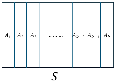
Figure 2.5: A partition of the sample space.

Then for any other event $B$,
\[ \begin{split} P(B)& = P(B\cap A_1)+P(B\cap A_2)+\cdots+P(B\cap A_k) \\ &=P(B \mid A_1)P(A_1)+P(B \mid A_2)P(A_2)+\cdots+P(B \mid A_k)P(A_k) \\ &= \sum_{i=1}^k P(B\mid A_i)P(A_i) \end{split} \]

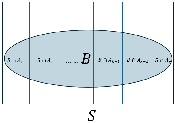
Figure 2.6: Law of total probability.

Bayes’ Rule

For event $A$ and $B$, where $P(B)\ne 0$, \[ P(A\mid B)=\frac{P(B\mid A)P(A)}{P(B)} . \]

2.11 Independence

Two events $A$ and $B$ are independent if $P(A\mid B)=P(A)$ and are dependent otherwise.

It is also straightforward to show that if $A$ and $B$ are independent, then so are the following pairs of events:

$A^c$ and $B$,
$A$ and $B^c$, and
$A^c$ and $B^c$.

$A$ and $B$ are independent if and only if (iff)
\[ P(A \cap B)=P(A)\cdot P(B) \]

Recall of multiplication rule: $P(A \cap B)=P(A \mid B)\cdot P(B)$.

If the joint probability of event $A$ and $B$ is equal to the product of their corresponding probabilities, then these two events are independent.

Independence of More Than Two Events

Events $A_1, \ldots, A_n$ are mutually independent if for every and every subset of indices $i_1, i_2, . . . , i_k$,
\[ P(A_{i_1}\cap A_{i_2}\cap \ldots\cap A_{i_k})=P(A_{i_1})\cdot P(A_{i_2}) \cdots P(A_{i_k}) \] the events are mutually independent if the probability of the intersection of any subset of the n events is equal to the product of the individual probabilities.

In using the multiplication property for more than two independent events, it is legitimate to replace one or more of the by their complements (e.g., if $A_1$, $A_2$, and $A_3$ are independent events, so are $A_1^c$, $A_2^c$ , and $A_3^c$).

Beware that “mutually exclusive” does not imply “independence”. On the contrary, two mutually exclusive events are dependent!