Chapter 10 Hypothesis Testing on Two Samples
Assumptions:
- \(X_1, X_2,\ldots, X_m\) is a random sample from a population with mean \(\mu_1\) and variance \(\sigma_1^2\).
- \(Y_1, Y_2,\ldots, Y_n\) is a random sample from another population with mean \(\mu_2\) and variance \(\sigma^2_2\).
- The \(X\) and \(Y\) samples are independent of one another.
Question:
- are \(\mu_1\) and \(\mu_2\) statistically different?
- If they are different, which one is larger?
The first question can be formulated into hypotheses as “\(H_0: \mu_1-\mu_2=0\) vs \(H_a: \mu_1-\mu_2 \ne 0\)”;
The second question can be formulated as “\(H_0: \mu_1-\mu_2=0\) vs \(H_a: \mu_1-\mu_2 > 0\)” or “\(H_0: \mu_1-\mu_2=0\) vs \(H_a: \mu_1-\mu_2 < 0\)”;
Let’s consider “\(H_0: \mu_1-\mu_2=0\) vs \(H_a: \mu_1-\mu_2 \ne 0\)” first.
First step of hypothesis testing is to find a proper test statistic, which is usually based on the estimator of parameters in the hypotheses. Here, we are testing about \(\mu_1-\mu_2\), so the natural estimator is \(\bar X-\bar Y\).
From the previous chapter about one sample tests, we already know the sampling distribution of \(\bar X\) and \(\bar Y\), which are \[ \bar X\sim N \left(\mu_1, \sigma_1/\sqrt{m} \right) \] \[ \bar Y\sim N \left(\mu_2, \sigma_2/\sqrt{n} \right) \] According to the properties of normal distributions, \(\bar X-\bar Y\) is also normally distributed and \[ E(\bar X-\bar Y)=\mu_1-\mu_2 \] \[ V(\bar X-\bar Y)=\frac{\sigma^2_1}{m}+\frac{\sigma^2_2}{n} \] which can be summarized as \[ \left(\bar X-\bar Y\right) \sim N\left(\mu_1-\mu_2,\sqrt{\frac{\sigma^2_1}{m}+\frac{\sigma^2_2}{n}}\right). \] Thus, we can form the test statistic as \[ \frac{(\bar X-\bar Y)-(\mu_1-\mu_2)}{\sqrt{\frac{\sigma^2_1}{m}+\frac{\sigma^2_2}{n}}}. \]
10.1 Z-test of two population means (two-sided)
If the standard deviations \(\sigma_1\) and \(\sigma_2\) are known, under the null hypothesis \(H_0: \mu_1-\mu_2=0\), The test statistic has standard normal distribution \[ Z=\frac{(\bar X-\bar Y)-(\mu_1-\mu_2)}{\sqrt{\frac{\sigma^2_1}{m}+\frac{\sigma^2_2}{n}}}=\frac{\bar X-\bar Y}{\sqrt{\frac{\sigma^2_1}{m}+\frac{\sigma^2_2}{n}}} \sim N(0, 1). \] Decision rules
We reject \(H_0\), if the value of test statistic calculated from the two sample means \(\bar x\) and \(\bar y\) is less than \(-z_{\alpha/2}\) or greater than \(z_{\alpha/2}\), where \(\alpha\) is the level of significance.
The rejection region can be expressed as \[ \frac{\bar x-\bar y}{\sqrt{\frac{\sigma^2_1}{m}+\frac{\sigma^2_2}{n}}}<-z_{\alpha/2} \;\;\;\text{or}\;\;\; \frac{\bar x-\bar y}{\sqrt{\frac{\sigma^2_1}{m}+\frac{\sigma^2_2}{n}}}>z_{\alpha/2} . \]
P-value
If we observed difference in sample means are \(\bar x-\bar y\), then the currently observed test statistic is \[ z=\frac{\bar x-\bar y}{\sqrt{\frac{\sigma^2_1}{m}+\frac{\sigma^2_2}{n}}} \]
the p-value will be \[ \begin{split} P\left(Z< - |z| \text{ or } Z>|z| \right) &= P\left(Z< - \frac{\left|\bar x-\bar y\right|}{\sqrt{\frac{\sigma^2_1}{m}+\frac{\sigma^2_2}{n}}} \right)+P\left( Z> \frac{\left|\bar x-\bar y\right|}{\sqrt{\frac{\sigma^2_1}{m}+\frac{\sigma^2_2}{n}}}\right) \\ &=2P\left( Z> \frac{\left|\bar x-\bar y\right|}{\sqrt{\frac{\sigma^2_1}{m}+\frac{\sigma^2_2}{n}}}\right) \\ &=2\left(1-\Phi\left(\frac{\left|\bar x-\bar y\right|}{\sqrt{\frac{\sigma^2_1}{m}+\frac{\sigma^2_2}{n}}}\right)\right) \end{split} \]
10.2 Z-test of two population means (right-sided)
If we want to test \[ H_0: \mu_1-\mu_2=0 \text{ vs } H_a: \mu_1-\mu_2 > 0 \] The test statistic is the same with the two-sided test, under the null hypothesis \(H_0: \mu_1-\mu_2=0\), The test statistic has standard normal distribution \[ Z=\frac{\bar X-\bar Y}{\sqrt{\frac{\sigma^2_1}{m}+\frac{\sigma^2_2}{n}}} \sim N(0, 1). \] Decision rules:
We reject \(H_0\), if the value of test statistic calculated from the two sample means \(\bar x\) and \(\bar y\) is greater than \(z_{\alpha}\), where \(\alpha\) is the level of significance. \[ \frac{\bar x-\bar y}{\sqrt{\frac{\sigma^2_1}{m}+\frac{\sigma^2_2}{n}}}>z_{\alpha} \] \[ \Downarrow \] \[ \bar x-\bar y>z_{\alpha} \sqrt{\frac{\sigma^2_1}{m}+\frac{\sigma^2_2}{n}} \] P-value
If we observed difference in sample means are \(\bar x-\bar y\), the p-value will be \[ P\left(Z> \frac{\bar x-\bar y}{\sqrt{\frac{\sigma^2_1}{m}+\frac{\sigma^2_2}{n}}}\right) \]
10.3 Z-test of two population means (left-sided)
If we want to test \[ H_0: \mu_1-\mu_2=0 \text{ vs } H_a: \mu_1-\mu_2 < 0 \] Decision rules:
We reject \(H_0\), if the value of test statistic calculated from the two sample means \(\bar x\) and \(\bar y\) is less than \(-z_{\alpha}\), where \(\alpha\) is the level of significance. \[ \frac{\bar x-\bar y}{\sqrt{\frac{\sigma^2_1}{m}+\frac{\sigma^2_2}{n}}}<-z_{\alpha} \\ \Downarrow \\ \bar x-\bar y<-z_{\alpha} \sqrt{\frac{\sigma^2_1}{m}+\frac{\sigma^2_2}{n}} \] P-value
If we observed difference in sample means are \(\bar x-\bar y\), the p-value will be \[ P\left(Z< \frac{\bar x-\bar y}{\sqrt{\frac{\sigma^2_1}{m}+\frac{\sigma^2_2}{n}}}\right) \]
10.4 Generalization to \(H_0: \mu_1-\mu_2=\Delta\)
The previous cases are special cases for \(\Delta=0\). If we already know there exists difference between two population means, and want to see whether or not the difference is equal to \(\Delta\), we can formulate the hypotheses as \[ H_0: \mu_1-\mu_2=\Delta \text{ vs } H_a: \mu_1-\mu_2\ne \Delta \] For one-sided tests, the alternative hypothesis can be \(H_a: \mu_1-\mu_2< \Delta\) or \(H_a: \mu_1-\mu_2> \Delta\).
We can move the \(\Delta\) to the left side of the inequation, and those hypotheses become \[ H_0: \mu_1-\mu_2-\Delta=0 \text{ vs } H_a: \mu_1-\mu_2- \Delta \ne 0 \] and \(H_a: \mu_1-\mu_2-\Delta< 0\) or \(H_a: \mu_1-\mu_2-\Delta> 0\) for one-sided tests.
In such case, we have to use the general form of the test statistic that we introduced in the very beginning, \[ \frac{(\bar X-\bar Y)-(\mu_1-\mu_2)}{\sqrt{\frac{\sigma^2_1}{m}+\frac{\sigma^2_2}{n}}}=\frac{(\bar X-\bar Y)-\Delta}{\sqrt{\frac{\sigma^2_1}{m}+\frac{\sigma^2_2}{n}}}. \] Under the null hypothesis \(H_0: \mu_1-\mu_2-\Delta=0\), the test statistic has standard normal distribution \[ Z=\frac{(\bar X-\bar Y)-\Delta}{\sqrt{\frac{\sigma^2_1}{m}+\frac{\sigma^2_2}{n}}} \sim N(0, 1). \] The decision rules and p-value calculations are the same with the special case.
10.5 Summary of z-test for two population means
| Tests | two-sided | left-side | right-side |
|---|---|---|---|
| Hypotheses | \(H_0: \mu_1-\mu_2=\Delta\) vs \(H_a: \mu_1-\mu_2\ne \Delta\) | \(H_0: \mu_1-\mu_2=\Delta\) vs \(H_a: \mu_1-\mu_2< \Delta\) | \(H_0: \mu_1-\mu_2=\Delta\) vs \(H_a: \mu_1-\mu_2> \Delta\) |
| Test statistic | \(Z=\frac{(\bar X-\bar Y)-\Delta}{\sqrt{\frac{\sigma^2_1}{m}+\frac{\sigma^2_2}{n}}}\) | \(Z=\frac{(\bar X-\bar Y)-\Delta}{\sqrt{\frac{\sigma^2_1}{m}+\frac{\sigma^2_2}{n}}}\) | \(Z=\frac{(\bar X-\bar Y)-\Delta}{\sqrt{\frac{\sigma^2_1}{m}+\frac{\sigma^2_2}{n}}}\) |
| Decision rule | Reject \(H_0\) if the observed \(z\) is less than \(-z_{\alpha/2}\) or greater than \(z_{\alpha/2}\) | Reject \(H_0\) if the observed \(z\) is less than \(-z_{\alpha}\) | Reject \(H_0\) if the observed \(z\) is greater than \(z_{\alpha}\) |
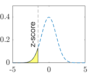
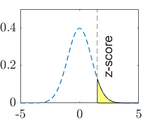
| P-value | \(2\left(1-\Phi\left(\frac{\left|\bar x-\bar y-\Delta\right|}{\sqrt{\frac{\sigma^2_1}{m}+\frac{\sigma^2_2}{n}}}\right)\right)\) | \(\Phi\left(\frac{\bar x-\bar y-\Delta}{\sqrt{\frac{\sigma^2_1}{m}+\frac{\sigma^2_2}{n}}}\right)\) | \(1-\Phi\left(\frac{\bar x-\bar y-\Delta}{\sqrt{\frac{\sigma^2_1}{m}+\frac{\sigma^2_2}{n}}}\right)\) |
| P-value (graphic) | 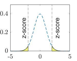 |
 |
 |
Note: \(\Delta\) is a specific number and \(\alpha\) is the level of significance.
z-score: Once we collected data points and calculated sample means, they are two specific numbers, which are denoted by lowercase \(\bar x\) and \(\bar y\). The calculated value of test statistic is called z-score, which is an instance of the test statistic for a specific data set, \[ z=\frac{(\bar x-\bar y)-\Delta}{\sqrt{\frac{\sigma^2_1}{m}+\frac{\sigma^2_2}{n}}}. \]
10.6 T-tests between two population means
In practice, we usually do not know population standard deviations. Without the knowledge of \(\sigma_1\) and \(\sigma_2\), we will not be able to form the test statistic \[ Z=\frac{(\bar X-\bar Y)-\Delta}{\sqrt{\frac{\sigma^2_1}{m}+\frac{\sigma^2_2}{n}}}. \] Instead, the values of \(\sigma_1\) and \(\sigma_2\) have to be estimated by their estimators, which are sample standard deviations, denoted by \(S_1\) and \(S_2\). Thus, the test statistic becomes \[ T=\frac{(\bar X-\bar Y)-\Delta}{\sqrt{\frac{S^2_1}{m}+\frac{S^2_2}{n}}}, \] which has approximately \(t\)-distribution with degrees of freedom estimated by \[ \nu=\frac{\left(\frac{S_1^2}{m}+\frac{S_2^2}{n}\right)^2}{\frac{(S_1^2/m)^2}{m-1}+\frac{(S_2^2/n)^2}{n-1}}. \] If \(\nu\) is not an integer, round it down to the nearest integer.
For \(t\)-tests, the instances of the test statistic (after evaluated by a specific sample) are called \(t\)-scores \[ t=\frac{(\bar x-\bar y)-\Delta}{\sqrt{\frac{s^2_1}{m}+\frac{s^2_2}{n}}}. \]
10.7 Summary of t-test for two population means
| Tests | two-sided | left-side | right-side |
|---|---|---|---|
| Hypotheses | \(H_0: \mu_1-\mu_2=\Delta\) vs \(H_a: \mu_1-\mu_2\ne \Delta\) | \(H_0: \mu_1-\mu_2=\Delta\) vs \(H_a: \mu_1-\mu_2< \Delta\) | \(H_0: \mu_1-\mu_2=\Delta\) vs \(H_a: \mu_1-\mu_2> \Delta\) |
| Test statistic | \(T=\frac{(\bar X-\bar Y)-\Delta}{\sqrt{\frac{S^2_1}{m}+\frac{S^2_2}{n}}}\) | \(T=\frac{(\bar X-\bar Y)-\Delta}{\sqrt{\frac{S^2_1}{m}+\frac{S^2_2}{n}}}\) | \(T=\frac{(\bar X-\bar Y)-\Delta}{\sqrt{\frac{S^2_1}{m}+\frac{S^2_2}{n}}}\) |
| Decision rule | Reject \(H_0\) if observe \(t<-t_{\alpha/2,\nu}\) or \(t>t_{\alpha/2, \nu}\) | Reject \(H_0\) if observe \(t<-t_{\alpha,\nu}\) | Reject \(H_0\) if the observed \(t>t_{\alpha,\nu}\) |
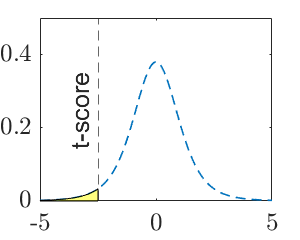
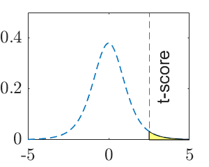
| P-value | \(2\left(1-F_\nu\left(\frac{\left|\bar x-\bar y-\Delta\right|}{\sqrt{\frac{s^2_1}{m}+\frac{s^2_2}{n}}}\right)\right)\) | \(F_\nu\left(\frac{\bar x-\bar y-\Delta}{\sqrt{\frac{s^2_1}{m}+\frac{s^2_2}{n}}}\right)\) | \(1-F_\nu\left(\frac{\bar x-\bar y-\Delta}{\sqrt{\frac{s^2_1}{m}+\frac{s^2_2}{n}}}\right)\) |
| P-value (graphic) | 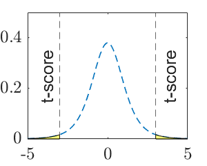 |
 |
 |
Note: \(F_\nu\) is the cdf of t-distribution with \(\nu\) degrees of freedom, where \(\nu=\frac{\left(\frac{s_1^2}{m}+\frac{s_2^2}{n}\right)^2}{\frac{(s_1^2/m)^2}{m-1}+\frac{(s_2^2/n)^2}{n-1}}\), (round \(\nu\) down to the nearest integer).
Special case when \(\sigma_1=\sigma_2\)
In many situations, two populations are assumed to have equal variances, though the variances are unknown. In such case, the test statistic for the t-test will be \[ T=\frac{(\bar X-\bar Y)-\Delta}{S_p}, \] where the \(S_p\) is the pooled estimator of the population standard deviation and it is calculated by \[ S^2_p=\frac{m-1}{m+n-2}\cdot S_1^2+\frac{n-1}{m+n-2}\cdot S_2^2 \] The t-test procedures will be exactly the same after replacing \(\sqrt{\frac{S^2_1}{m}+\frac{S^2_2}{n}}\) with \(S_p\).
10.8 Hypothesis Testing and Confidence Intervals
| Type of Tests | Hypotheses | Acceptance Region | Confidence Interval for the true \(\Delta\) |
|---|---|---|---|
| z | \(H_0: \mu_1-\mu_2=\Delta\) vs \(H_a: \mu_1-\mu_2\ne \Delta\) | \(-z_{\alpha/2}<\frac{(\bar X-\bar Y)-\Delta}{\sqrt{\frac{\sigma^2_1}{m}+\frac{\sigma^2_2}{n}}}<z_{\alpha/2}\) | \(\left[(\bar x-\bar y)\pm z_{\alpha/2}\cdot\sqrt{\frac{\sigma^2_1}{m}+\frac{\sigma^2_2}{n}}\right]\) |
| z | \(H_0: \mu_1-\mu_2=\Delta\) vs \(H_a: \mu_1-\mu_2< \Delta\) | \(\frac{(\bar X-\bar Y)-\Delta}{\sqrt{\frac{\sigma^2_1}{m}+\frac{\sigma^2_2}{n}}}>-z_\alpha\) | \(\left(-\infty,\; (\bar x-\bar y)+z_{\alpha}\cdot\sqrt{\frac{\sigma^2_1}{m}+\frac{\sigma^2_2}{n}}\right]\) |
| z | \(H_0: \mu_1-\mu_2=\Delta\) vs \(H_a: \mu_1-\mu_2- \Delta > 0\) | \(\frac{(\bar X-\bar Y)-\Delta}{\sqrt{\frac{\sigma^2_1}{m}+\frac{\sigma^2_2}{n}}}<z_\alpha\) | \(\left[(\bar x-\bar y)-z_{\alpha}\cdot\sqrt{\frac{\sigma^2_1}{m}+\frac{\sigma^2_2}{n}}, \;\infty \right)\) |
| t | \(H_0: \mu_1-\mu_2=\Delta\) vs \(H_a: \mu_1-\mu_2\ne \Delta\) | \(-t_{\alpha/2,\nu}<\frac{(\bar X-\bar Y)-\Delta}{\sqrt{\frac{\sigma^2_1}{m}+\frac{\sigma^2_2}{n}}}<t_{\alpha/2,\nu}\) | \(\left[(\bar x-\bar y)\pm t_{\alpha/2, \nu}\cdot\sqrt{\frac{s^2_1}{m}+\frac{s^2_2}{n}}\right]\) |
| t | \(H_0: \mu_1-\mu_2=\Delta\) vs \(H_a: \mu_1-\mu_2< \Delta\) | \(\frac{(\bar X-\bar Y)-\Delta}{\sqrt{\frac{\sigma^2_1}{m}+\frac{\sigma^2_2}{n}}}>-t_{\alpha,\nu}\) | \(\left(-\infty,\;(\bar x-\bar y)+t_{\alpha, \nu}\cdot\sqrt{\frac{s^2_1}{m}+\frac{s^2_2}{n}}\right]\) |
| t | \(H_0: \mu_1-\mu_2=\Delta\) vs \(H_a: \mu_1-\mu_2- \Delta > 0\) | \(\frac{(\bar X-\bar Y)-\Delta}{\sqrt{\frac{\sigma^2_1}{m}+\frac{\sigma^2_2}{n}}}<t_{\alpha, \nu}\) | \(\left[(\bar x-\bar y)-t_{\alpha,\nu}\cdot\sqrt{\frac{s^2_1}{m}+\frac{s^2_2}{n}}, \infty\right)\) |
Note: for t-test with equal variance \(\sigma_1=\sigma_2\), replace the \(\sqrt{\frac{S^2_1}{m}+\frac{S^2_2}{n}}\) with pooled sample standard deviation \(S_p=\sqrt{\frac{m-1}{m+n-2}\cdot S_1^2+\frac{n-1}{m+n-2}\cdot S_2^2}\).