Chapter 8 Interval Estimation

8.1 Review

• Parameters are fixed values that describe the distribution of a population, for example, the mean (also called the expected value) describes the center of a distribution while the standard deviation describes the degree of variation.

• A statistic is a random variable whose value depends on the sample. A statistic is used to estimate a parameter. For example, the sample mean \(\bar X\) is the statistic used as an estimator for the population mean \(\mu\).

• The probability distribution of a statistic is called sampling distribution.

In most situations, a point estimation does not provide enough information of a parameter. Investigators may also want to know the goodness the point estimation is. For example, if you estimate a person’s age, you might give a range, such as “he is in \(30\)s”, instead a single number \(33\). The range with a reasonable span, such as \(10\) years, makes more sense than a range like \(0-100\).

When we the estimation for a parameter is a range, we call this as “Interval Estimation”.

Interval estimation is often centered on a point estimation, and with a margin on both side. For example, The point estimation of a person’s age is \(33\), then the interval estimation can be \(33\pm5\), which is \([28, 38]\). The interval is called “Confidence Interval (CI)”, and the half width of the interval is sometimes called the “Margin of Error”. CIs are derived from the sampling distribution of a point estimator.

In this Chapter, we first look at the CI for a population mean.

8.2 Assumptions

Suppose that the parameter of interest is a population mean \(\mu\) and that

1. The population is normally distributed (Normality assumption) ;

2. The population standard deviation \(\sigma\) is known.

The sampling distribution of the sample mean \(\bar X\) is normal with expected value \(\mu\) and standard deviation \(\sigma/\sqrt n\), where \(n\) is the sample size. This can be denoted as \[ \bar X\sim N\left(\mu, \frac{\sigma}{\sqrt n}\right). \]

8.3 CI for Population Mean

After the standardization on \(\bar X\), we have \[ Z=\frac{\bar X-\mu}{\sigma/\sqrt n} \sim N(0, 1). \] We denote the left side as \(Z\), which is a conventional notation for a standard normal rv.

For the standard normal distribution, we have \[ P(-1.96<Z<1.96)=0.95 \] as is shown in Figure 8.1.

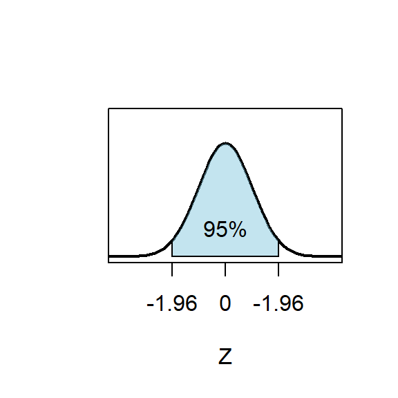
Figure 8.1: Standard normal distribution

In other words, \[ P\left(-1.96<\frac{\bar X-\mu}{\sigma/\sqrt n} <1.96\right)=0.95 \] \[ \Downarrow \] \[ P\left(\bar X-1.96\cdot \frac{\sigma}{\sqrt n}<\mu <\bar X+1.96\cdot \frac{\sigma}{\sqrt n}\right)=0.95 \] This equation “seems” to say that the interval \((\bar X-1.96\cdot \frac{\sigma}{\sqrt n},\;\bar X+1.96\cdot \frac{\sigma}{\sqrt n})\) “catch” the true value of \(\mu\) with the probability of \(0.95\). This interval is called the confidence interval (CI) for \(\mu\) and the confidence level is \(95\%\).

If we take a closer look at the CI, we will see its two “brackets” are not fixed values. Remember that the statistic \(\bar X\) is a random variable, so are \(\bar X\pm 1.96\cdot {\sigma}/{\sqrt n}\), of course. However, the confidence interval has a fixed width, which is \(2\times 1.96\cdot {\sigma}/{\sqrt n}={3.92\sigma}/{\sqrt n}\).

In conclusion, the interval \((\bar X-1.96\cdot {\sigma}/{\sqrt n},\;\bar X+1.96\cdot {\sigma}/{\sqrt n})\) is a random interval with a fixed width. We can interpret this CI as: If we collect \(100\) samples from the population, each sample will give us a different interval and approximately \(95\%\) of those will “capture” the true value of \(\mu\).

8.4 CIs of Other Confidence Level

With the same setting, if we want the confidence level of \(99\%\) instead of \(95\%\), what should we do?

The \(99\%\) CI can also be derived from the sampling distribution \[ Z=\frac{\bar X-\mu}{\sigma/\sqrt n} \sim N(0, 1). \] For the standard normal distribution, \[ P\left(-\color{red}{2.58}\color{black}<Z<\color{red}{2.58}\right)=\color{red}{0.99} \] as is seen in Figure 8.2.

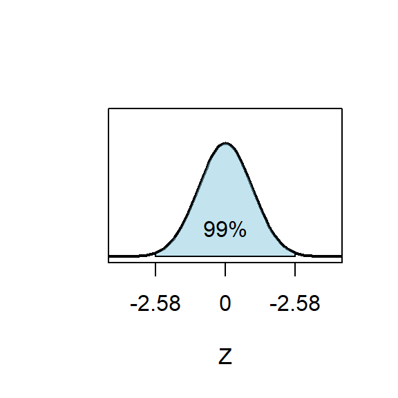
Figure 8.2: Standard normal distribution

Thus, \[ P\left(-\color{red}{2.58}\color{black}<\frac{\bar X-\mu}{\sigma/\sqrt n} <\color{red}{2.58}\right)=\color{red}{0.99} \] \[ \Downarrow \] \[ P\left(\bar X-\color{red}{2.58}\color{black}\cdot \frac{\sigma}{\sqrt n}<\mu <\bar X+\color{red}{2.58}\color{black}\cdot \frac{\sigma}{\sqrt n}\right)=\color{red}{0.99} \] The \(99\%\) CI for \(\mu\) is \((\bar X-\color{red}{2.58}\color{black}\cdot {\sigma}/{\sqrt n},\;\bar X+\color{red}{2.58}\color{black}\cdot {\sigma}/{\sqrt n})\).

We can see the only difference is the multiplier for \({\sigma}/{\sqrt n}\), changing from \(1.96\) to \(2.58\). In other words, the width of the confidence interval becomes \(2\times 2.58\cdot {\sigma}/{\sqrt n}={5.16\sigma}/{\sqrt n}\), which is wider than that of \(95\%\) CI.

Significance level: the significance level, often denoted by \(\alpha\), is defined by \(1\) minus the confidence level. In other words, the confidence level is \(1-\alpha\).

For an arbitrary confidence level \(1-\alpha\), the CI for the mean of a normal population is \[ \left(\bar X-\color{red}{z_{\alpha/2}}\color{black}\cdot \frac{\sigma}{\sqrt n},\;\bar X+\color{red}{z_{\alpha/2}}\color{black}\cdot \frac{\sigma}{\sqrt n}\right), \] where \(z_{\alpha/2}\) is the critical value for \(\alpha/2\).

Recall: \(z\) critical values:

The definition of \(z\) critical values are shown in Figure 8.3.

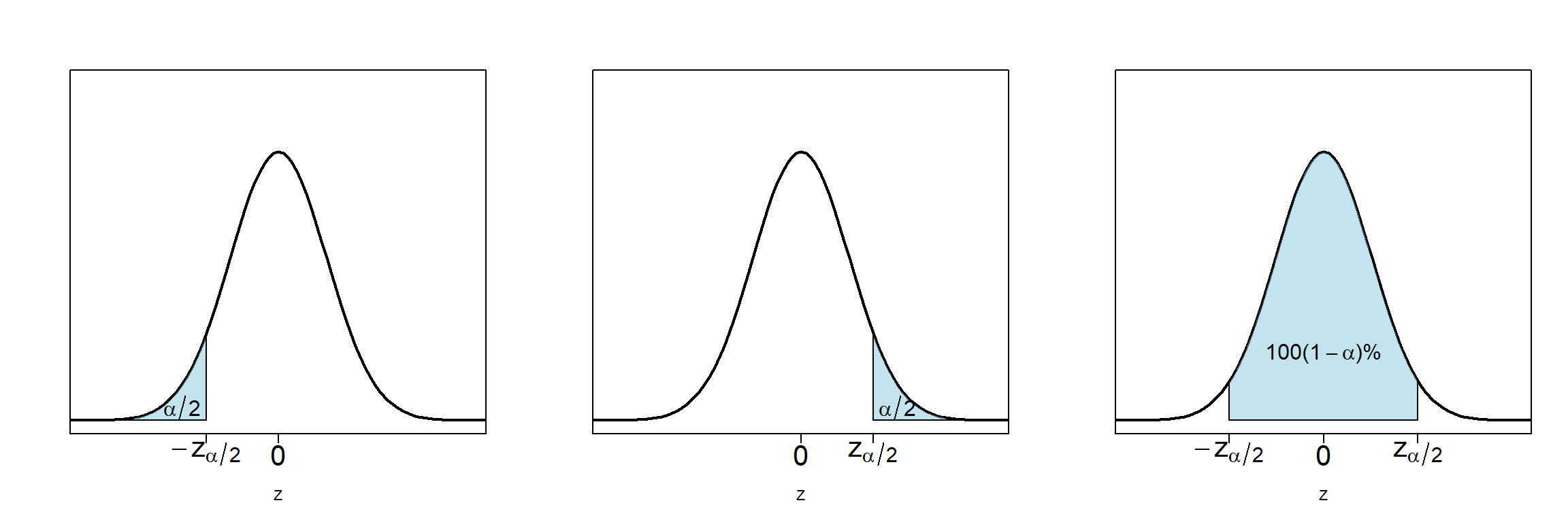
Figure 8.3: Standard normal distribution

Keep in mind that this is based on assumptions that the population has a normal distribution with a known standard deviation.

8.5 One-sided CIs

The confidence intervals we have seen by so far are called two-sided confidence intervals, which have both upper and lower limits.

In some cases, we are only interested in the upper or lower bound of the parameter. In such case, we will need one-sided confidence intervals.

For any confidence level \(1-\alpha\), one sided CIs for the mean of a normal population is \[ \left(\bar X-\color{red}{z_{\alpha}}\color{black}\cdot \frac{\sigma}{\sqrt n},\; \infty\right) \] and \[ \left(-\infty, \;\bar X+\color{red}{z_{\alpha}}\color{black}\cdot \frac{\sigma}{\sqrt n}\right) \] where \(z_\alpha\) is the critical value for \(\alpha\). They are derived in the similar way as the two-sided CI.

8.6 CI for Population Mean with unknown \(\sigma\)

In most cases, we will never know the population’s standard deviation. The value of \(\sigma\) must be estimated by the sample standard deviation \[ S=\sqrt{\frac{\sum_{i=1}^n (X_i-\bar X)^2}{n-1}}. \] In such case, the confidence intervals cannot be derived from the sampling distribution \[ Z=\frac{\bar X-\mu}{\sigma/\sqrt n} \sim N(0, 1), \] since the left side has another unknown quantity \(\sigma\) beside of the \(\mu\).

We replace \(\sigma\) by its estimator \(S\), so that we have a new random variable \[ T=\frac{\bar X-\mu}{S/\sqrt n}, \] which has \(t\)-distribution with \(n-1\) degrees of freedom.

Since the sampling distribution becomes \[ T=\frac{\bar X-\mu}{S/\sqrt n} \sim t_{\nu=n-1}, \] we have

\[ P\left( - \color{red}{t_{\alpha/2, n-1}}\color{black}<\frac{\bar X-\mu}{S/\sqrt n} <\color{red}{t_{\alpha/2, n-1}}\right)=\color{red}{1-\alpha} \] \[ \Downarrow \] \[ P\left(\bar X-\color{red}{t_{\alpha/2, n-1}}\color{black}\cdot \frac{S}{\sqrt n}<\mu <\bar X+\color{red}{t_{\alpha/2, n-1}}\color{black}\cdot \frac{S}{\sqrt n}\right)=\color{red}{1-\alpha}. \] The two sided CI for \(\mu\) is \[ (\bar X-\color{red}{t_{\alpha/2, n-1}}\color{black}\cdot \frac{S}{\sqrt n},\;\bar X+\color{red}{t_{\alpha/2, n-1}}\color{black}\cdot \frac{S}{\sqrt n}), \] where \(t_{\alpha/2, n-1}\) is the \(t\) critical value for \(\alpha/2\) and \(n-1\) degrees of freedom.

\(t\) critical values:

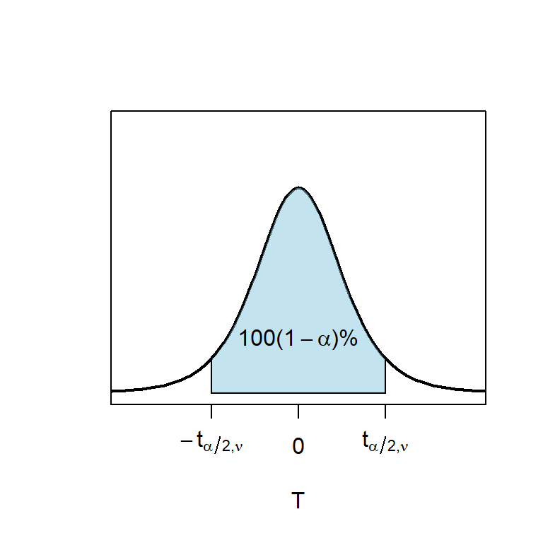
Figure 8.4: Student-t distribution

Similarly, one-sided CIs are

\[ \left(\bar X-\color{red}{t_{\alpha, n-1}}\color{black}\cdot \frac{S}{\sqrt n},\;\infty\right) \]

and

\[ \left(-\infty, \;\bar X+\color{red}{t_{\alpha, n-1}}\color{black}\cdot \frac{S}{\sqrt n}\right). \]

8.7 CIs for Large \(n\)

Remember, all confidence intervals we discussed are for normal populations. If the population is not normally distributed, we cannot easily find the sampling distribution of \(\bar X\) and will not be able to derive CIs for \(\mu\) accordingly.

Luckily, there are exceptions.

Recall of Central Limit Theorem: No matter what distribution family a population has, as long as the sample size is large enough, the sampling distribution of the sample mean \(\bar X\) will be approximately normal with expected value \(\mu\) and standard deviation \(\sigma/\sqrt n\).

In other word, for a large sample size, the normality assumption can be lifted and all the formulas for confidence intervals we derived before can be used for any population. Besides, when \(n\) is large, \(t\) critical values and \(z\) critical values are very similar, so we may simply use \(z_\alpha\) in place of \(t_{\alpha, n-1}\).

8.8 Interpretation of CI

For the sample population, with the same sampling scheme, different investigators may get different samples. Different samples will give different confidence intervals for the parameter, though they are computed with an identical procedure. Thus, as we mentioned, confidence intervals are random intervals with a fixed width. For example, investigator A have \(\bar x=5.2\) while investigator B have \(\bar x=4.9\) since they use different samples drawn from a same population. Of course, they will end up with two different CIs for the \(\mu\).

If investigators repeat the steps of obtaining the \(100(1-\alpha)\%\) CI on multiple different samples, there will be approximately \(100(1-\alpha)\%\) of those intervals capture the true value of parameter. This is the correct interpretation of CIs. Keep in mind that we should never interpret a single CI as an interval having \(100(1-\alpha)\%\) of the chance to contain the true parameter.

8.9 Summary

Here is the summary of confidence intervals for the mean of a normal population.

\(100(1-\alpha)\%\) CI for \(\mu\)	Known \(\sigma\)	Unknown \(\sigma\)	Large \(n\), Unknown \(\sigma\)
Two side	\((\bar X \pm\color{red}{z_{\alpha/2}}\color{black}\cdot {\sigma}/{\sqrt n})\)	\((\bar X\pm \color{red}{t_{\alpha/2, n-1}}\color{black}\cdot {S}/{\sqrt n})\)	\((\bar X\pm \color{red}{z_{\alpha/2}}\color{black}\cdot {S}/{\sqrt n})\)
Left side	\((\bar X-\color{red}z_{\alpha}\color{black}\cdot {\sigma}/{\sqrt n}, \; \infty)\)	\((\bar X-\color{red}{t_{\alpha, n-1}}\color{black}\cdot {S}/{\sqrt n},\;\infty)\)	\((\bar X-\color{red}{z_{\alpha}}\color{black}\cdot {S}/{\sqrt n},\;\infty)\)
Right side	\((-\infty,\;\bar X+\color{red}{z_{\alpha}}\color{black}\cdot {\sigma}/{\sqrt n})\)	\((-\infty,\; \bar X+\color{red}{t_{\alpha, n-1}}\color{black}\cdot {S}/{\sqrt n})\)	\((-\infty,\; \bar X+\color{red}{z_{\alpha}}\color{black}\cdot {S}/{\sqrt n})\)

Note: \(S\) is the sample standard deviation \(S=\sqrt{{\sum_{i=1}^n (X_i-\bar X)^2}/{(n-1)}}\).

8.10 CIs for other Parameters

8.10.1 CI for Population Proportion

Let \(p\) denote the proportion of “successes” in a population, where success identifies an individual or object that has a specified property. A random sample of \(n\) individuals is to be selected, and \(X\) is the number of successes in the sample. The sample proportion of successes \[ \hat p=\frac{X}{n} \] has approximately normal distribution with \(N\left(p, \sqrt{p(1-p)/n}\right)\).

After standardization, we have \[ \frac{\hat p-p}{\sqrt{p(1-p)/n}} \overset{approx}{\sim} N(0, 1). \] Thus, for the level of significance \(\alpha\), we have \[ P\left (-z_{\alpha/2}<\frac{\hat p-p}{\sqrt{p(1-p)/n}}<z_{\alpha/2}\right)\approx 1-\alpha. \] The inequation inside the parenthesis can not be easily transformed into a form like \(\cdots <p<\cdots\) , because the denominator also contains \(p\). It has to be dealt in another way. We first replace the \(<\) sign in the inequation with the \(=\) sign and solve the equation respect to \(p\). The equation \[ \frac{\hat p-p}{\sqrt{p(1-p)/n}}=z_{\alpha/2} \] can be rewritten into a quadratic equation by taking squares on both sides. Using quadratic formula, we obtain two roots \[ p = \frac{\hat p+\frac{z^2_{\alpha/2}}{2n}}{1+\frac{z^2_{\alpha/2}}{n}} \pm z_{\alpha/2}\cdot \frac{\sqrt{\frac{\hat p(1-\hat p)}{n}+\frac{z^2_{\alpha/2}}{4n^2}}}{1+\frac{z^2_{\alpha/2}}{n}} \] which are the upper and lower bounds of \(100(1-\alpha)\%\) CI for the population proportion. This is often referred as the score CI for \(p\).

When the sample size \(n\) is very large, \(z^2/(2n)\) is negligible compared to \(\hat p\) , \(z^2/n\) is negligible compared to \(1\), and also \(z^2/2n^2\) is negligible compared to \(\hat p(1-\hat p)/n\). In such case, the score interval is approximately \[ \hat p \pm z_{\alpha/2}\sqrt {\hat p(1-\hat p)}. \] However, the simplified form does not perform as well as the score CI, especially when the true \(p\) is around \(0\) or \(1\). The coverage probability, which is the probability that the random interval includes the actual value of \(p\), will be lower than the aimed confidence level \(100(1-\alpha)\%\).

8.10.2 CIs for Population Variance

For a normal population, the rv \[ \frac{(n-1)S^2}{\sigma^2}=\frac{\sum_{i=1}^n(X_i-\bar X)^2}{\sigma^2} \] has a chi-squared \(\chi^2\) distribution with \(n-1\) degrees of freedom.

Chi-squared critical value:

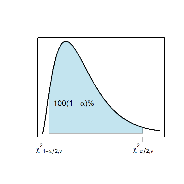
Figure 8.5: Chi-squared distribution

We can derive CI for \(\sigma^2\) from \[ P\left( \chi^2_{1-\alpha/2, \nu}<\frac{(n-1)S^2}{\sigma^2}<\chi^2_{\alpha/2, \nu}\right)=1-\alpha \] \[ \Downarrow \] \[ P\left( \frac{(n-1)S^2}{\color{red}{\chi^2_{\alpha/2, \nu}}}<{\sigma^2}<\frac{(n-1)S^2}{\color{red}{\chi^2_{1-\alpha/2, \nu}}}\right)=1-\alpha. \] So the \(100(1-\alpha)\%\) CI for the variance \(\sigma^2\) of a normal population is \[ \left(\frac{(n-1)S^2}{\color{red}{\chi^2_{\alpha/2, \nu}}},\; \frac{(n-1)S^2}{\color{red}{\chi^2_{1-\alpha/2, \nu}}}\right). \] Beware that \(\chi^2\) distribution is not symmetric, so \(\chi^2_{1-\alpha/2, \nu}\) is not the inverse of \(\chi^2_{\alpha/2, \nu}\) (unlike \(t\)-distribution, \(t_{1-\alpha/2,\nu}=-t_{\alpha/2,\nu}\)).