Chapter 9 Hypothesis Testing on One Sample

9.1 Basic Framework

Definition of Hypothesis: A hypothesis is a research argument/statement that is subject to further proof.

Most scientific research starts with the establishment of a proper hypothesis,

such as the hypothesis “Remdesivir is effective to reduce the symptoms caused by Covid-19 virus”.

9.1.1 Formulation of Hypotheses

Once the scientist established the purpose of the research activity, the research aim can be formulated by a set of hypotheses that contains two hypotheses contradictory to each other.

One is called the null hypothesis, denoted by \(H_0\), and another is called alternative hypothesis, denoted by \(H_a\).

For example, if the research aim is tell whether or not Remdesivir is effect to treat Covid-19 symptoms, scientists can test on the so-called length of stay in hospitalized patients infected by Covid-19. “Length of Stay (LOS)” means the time that a patient spend in the hospital facility before getting discharged. Let \(t_1\) be the mean LOS of treated group (with Remdesivir) and \(t_0\) be the mean LOS of the control group (treated by Placebo).

The pair of hypotheses can be \[ H_0: t_1=t_0 \text{ (Remdesivir has no effect)} \text{ vs } H_a: t_1<t_0 \text{ (Remdesivir has effect)} \] You may have noticed that we put the hypothesis that scientists want to prove in \(H_a\). The reason of doing this is related to the power of hypothesis that we will discuss about later.

The alternative hypothesis \(H_a\) is also called the “research hypothesis”, which implies the research statement that the research want to validate. On the other hand, the null hypothesis is the one that researchers want to reject.

In fact, the \(H_a\) defines the set of hypotheses used in research activities. Once the \(H_a\) is established, the null hypothesis is often implied.

For example,

1. \(H_a: \mu>0\) (in which case the implicit null hypothesis is \(\mu \le 0\))
2. \(H_a: \mu\ne0\) (in which case the implicit null hypothesis is \(\mu = 0\))

9.1.2 Test Procedure and P-values

After the formulation of hypotheses, we need to test them.

The first step is to find out the “test statistic” according to the hypotheses.

For example, given a normally distributed population with known standard deviation \(\sigma\), if we want to test whether or not the population mean \(\mu\) is equal to \(15\), we can form the hypotheses as

\(H_0: \mu=15\) vs \(H_a: \mu\ne 15\)

Next step is to find a statistic to test these hypotheses. From the Chapter of Interval Estimation, we already know the statistic related to the population mean is the sample mean \(\bar X\). For normally distributed population, the sample mean has sampling distribution \[ \bar X\sim N(\mu, \sigma/\sqrt n) \] Thus, under the null hypothesis (if \(H_0\) is true), the sampling distribution of \(\bar X\) should be \[ \bar X\sim N(15, \sigma/\sqrt n) \]

If we are going to collect \(n=10\) observations, and the population standard deviation is known to be \(\sigma=1\), the sampling distribution would be \(\bar X\sim N(15, 1/\sqrt 10)\) under the null hypothesis, as is seen in Figure 9.1.

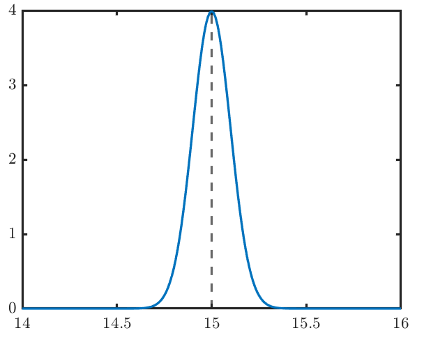
Figure 9.1: Sampling distribution under H0

Once we collected the observations, and calculated the sample mean \(\bar x=AVG(x_1, \ldots, x_{10})\), the value of \(\bar x\) will be around \(15\) if \(H_0\) is true. On the other hand, if the obtained \(\bar x\) is actually far way from \(15\) (such as \(\bar x <14.4\) or \(\bar x>15.6\)), the null hypothesis is very likely to be false.

9.1.3 Significance Level

Definition of small probability events/extreme events: given a hypothesis, if an event is unlikely to happen, it is called small probability event or extreme event for that hypothesis.

In the previous example, the event of \((\bar x<14.4\) or \(\bar x >15.6)\) is a small probability event for the null hypothesis \(H_0:\mu=15\).

Definition of Significance Level: Significance level defines how small the probability of extreme events should be treated as a small probability event. The significance level is often denoted by \(\alpha\). Commonly, \(\alpha\) can be equal to \(0.05\), \(0.1\), or \(0.001\).

In the previous example, under the null hypothesis, the probability of the event of \(\bar x<14.4\) or \(\bar x >15.6\) is \[ \alpha=P(\bar x<14.4 \mid \bar x >15.6)=0.05 \] In statistics, we assume that the small probability event/extreme event should not happen in the experiment. If it does happen, we conclude that the null hypothesis is false and reject it.

We have two ways to tell if the small probability event happens.

9.1.4 Rejection Region

One way is through so-called “rejection region”.

For the previous example, under the null hypothesis, we have \(\bar X\sim N(15, 1/\sqrt 10)\), thus \[ \frac{\bar X-15}{1/\sqrt 10}\sim N(0, 1) \] so \[ P(-1.96<\frac{\bar X-15}{1/\sqrt 10}<1.96)=1-\alpha=0.95 \] and \[ P(15-1.96/\sqrt 10<\bar X<15+1.96/\sqrt 10)=1-\alpha=0.95 \\ P(14.4<\bar X<15.6)=1-\alpha=0.95 \] If the observed sample mean \(\bar x=AVE(x_1,\ldots, x_{10})\) is somehow outside the range \((14.4, 15.6)\), the null hypothesis is likely to be false and should be rejected.

In other words, if the observed \(\bar x\) falls into the intervals \((-\infty, 14.4]\) and \([15.6, \infty)\), we reject \(H_0\). These two intervals combined is called “Rejection Region” for \(H_0\). Once the test statistic falls into the rejection region of \(H_0\), \(H_0\) gets rejected. Besides, the interval \((14.5, 15.6)\) is called “Acceptance Region”.

9.1.5 P-values

Another way to tell whether or not a small probability event is happening is through so-called “p-values”.

P-value is a probability that can be calculated AFTER we already observed the value of a test statistic.

P-value is the probability of events that are more extreme than the current observed one.

What does it mean by “more extreme”?

In the previous example, the test statistic is supposed to be around \(15\), if the \(H_0\) is true.

If the observed \(\bar x\) is far away from \(15\), it is treated as extreme. The more it deviates from \(\mu=15\), the more extreme it is.

If we observed \(\bar x=15.5\), it deviates from \(15\) by \(0.5\). The events that are “more extreme than this” is defined by observing \(\bar x\) that deviates from \(15\) by more than \(0.5\), which is \[ \bar X>15.5 \text{ or } \bar X<14.5. \] In such case, the p-value is defined by \[ P\left(\bar X>15.5 \text{ or } \bar X<14.5\right). \] Under the null hypothesis \(H_0\). \[ \begin{split} P(\bar X>15.5 \mid \bar x<14.5)&=1-P(14.5 \le \bar X \le 15.5) \\ &=1-P\left(\frac{14.5-15}{1/\sqrt 10} \le \frac{\bar X-15}{1/\sqrt 10} \le \frac{15.5-15}{1/\sqrt 10}\right) \\ &=1-P\left(-1.58\le \frac{\bar X-15}{1/\sqrt 10} \le 1.58\right) \\ &=1-P\left(-1.58\le Z \le 1.58\right) \\ &=1-\left(\Phi(1.58)-\Phi(-1.58)\right)=0.1142 \end{split} \]

If the p-value is less than the significance level \(\alpha\), then the \(H_0\) gets rejected, otherwise it is accepted.

We can see that p-value less than \(\alpha\) is equivalent to \(\bar x\) falls into the rejection region.

9.1.6 Type I and Type II errors

Type I error

We reject the null hypothesis once a small probability event under \(H_0\) is observed.

However, small probability events can happen under the null hypothesis, though the possibility is less than \(\alpha\).

When a small probability event happened and we rejected the null hypothesis but the \(H_0\) is actually true, we made so-called Type I error.

Type I error happens only when the decision is rejection and \(H_0\) is true.

The probability of committing Type I error is defined as \[ \alpha=P\left(\text{Rejection}\mid H_0 \text{ is true}\right) \] In the example we used previously, \[ \begin{split} P(\text{Rejection}\mid H_0 \text{ is true}) &=P(\bar x \text{ falls into rejection region}\mid H_0 \text{ is true}) \\ &=P(\bar X \le 14.5 \text{ or } \bar x \ge 15.6 \mid \mu=15) \\ &=\alpha \\ &=0.05 \end{split} \]

Type II error

Type II error happens when we fail to reject \(H_0\) when it is actually false.

Type II error happens only when the decision is acceptance.

The probability of committing Type II error is defined by \[ \beta=P(\text{Acceptance}\mid H_0 \text{ is false}) \] In the previous example, if the true population mean is \(\mu=16\) instead \(\mu=15\), the probability of making type II error is \[ \begin{split} P(\text{Acceptance}\mid H_0 \text{ is false}) &=P(\bar x \text{ falls into acceptance region}\mid H_0 \text{ is false}) \\ &=P(14.4<\bar X < 15.6 \mid \mu=16)\\ &=P\bigg(\frac{14.4-16}{1/\sqrt 10}<\frac{\bar X-16}{1/\sqrt 10} < \frac{15.6-16}{1/\sqrt 10} )\\ &=P\bigg(\frac{14.4-16}{1/\sqrt 10}<Z < \frac{15.6-10}{1/\sqrt 16} ) \\ &=\Phi(-1.26)-\Phi(-5.05) \\ &\approx 0.10 \end{split} \] You may notice that we need to know the true value of \(\mu\) to calculate the probability of type II error.

A little more notes about Type I and Type II errors:

Remember that we usually put something that we want to prove in \(H_a\), which is the research hypothesis.

When we make Type I error, we reject \(H_0\) and embrace \(H_a\) falsely, which means we proved something that is actually wrong.

When we make Type II error, we failed to reject \(H_0\) even though it is false. In other words, we failed to prove a true research hypothesis \(H_a\) and make no progress in the research activity.

Type I error is way more serious than the Type II error. In practice, we have more tolerance on type II error than on Type I error.

9.2 Tests on Population Mean

This section is about inference of population mean \(\mu\). The assumption is the population is normally distributed or approximately normally distributed.

We have two testing procedures named after the test statistics they used. If the test statistic is Z, then the hypothesis test is called z-test; If the test statistic is T, then the hypothesis test is called t-test.

Both z-test and t-test are based on the fact that the sample mean is normally distributed around the population mean, \[ \bar X\sim N\left(\mu, \sigma/\sqrt n\right) \] where \(\sigma\) is the population standard deviation and \(n\) is the sample size.

The hypotheses that we used in this section are \[ H_0: \mu=\mu_0 \text{ vs } H_a: \mu \ne \mu_0 \]

9.2.1 Z-tests

Z-tests are used when the population is normally distributed and the population standard deviation \(\sigma\) is known.

Given that \[ \bar X\sim N\left(\mu, \sigma/\sqrt n\right), \] and \(\sigma\) is known, we can form a test statistic \[ Z=\frac{\bar X-\mu}{\sigma/\sqrt n} \] which has standard normal distribution.

Assume that we want to test hypotheses \[ H_0: \mu=\mu_0 \text{ vs } H_a: \mu \ne \mu_0 \] and set the significance level \(\alpha=0.05\).

Under the hypothesis \(H_0: \mu=\mu_0\), we have \[ Z=\frac{\bar X-\mu_0}{\sigma/\sqrt n} \sim N(0, 1). \] According to the standard normal distribution, \[ P\left(-z_{\alpha/2} < Z < z_{\alpha/2}\right)=1-\alpha=0.95 \] \[ \Downarrow \] \[ P\left(-1.96 <\frac{\bar X-\mu_0}{\sigma/\sqrt n}<1.96\right)=0.95 \] \[ \Downarrow \] \[ P\left(\mu_0-1.96\cdot \frac{\sigma}{\sqrt n} <\bar X<\mu_0+1.96\cdot\frac{\sigma}{\sqrt n}\right)=0.95 \] Here we can see that the acceptance region is \[ \left(\mu_0-1.96\cdot \frac{\sigma}{\sqrt n}, \;\mu_0+1.96\cdot \frac{\sigma}{\sqrt n}\right) \] while the rejection region is \[ \left(-\infty, \mu_0-1.96\cdot \frac{\sigma}{\sqrt n}\right)\cup \left(\mu_0+1.96\cdot \frac{\sigma}{\sqrt n}, \infty\right) \]

Make conclusions:

After we collect the sample and calculated \(\bar x=AVG(x_1, \ldots, x_n)\), we reject \(H_0\) if \(\bar x\) is less than \(\mu_0-1.96\cdot \frac{\sigma}{\sqrt n}\) or greater than \(\mu_0+1.96\cdot \frac{\sigma}{\sqrt n}\), otherwise accept \(H_0\).

Calculate P-values:

Recall: P-value means the probability that the test statistic takes values that are more “extreme” than the one calculated from the current sample.

If the current sample mean is \(\bar x\), the calculated test statistic based on the current sample mean is \[ z=\frac{\bar x-\mu_0}{\sigma/\sqrt n} \] According to the \(H_0\), \(Z=\frac{\bar X-\mu_0}{\sigma/\sqrt n}\) has standard normal distribution and it should be distributed around zero. Thus, “extreme” means that it deviates from zero by large distance, so more extreme than the current calculated \(z\) implies \[ Z> |z| \] The p-value for the current \(z\) is \[ P(Z<-|z|)+P(Z>|z|)=2(1-\Phi(|z|)) \]

If the p-value is less than the significance level, then we reject the hypothesis \(H_0\).

9.2.2 T-tests

T-tests are used for normally distributed population with unknown standard deviation. Since the \(\sigma\) is unknown, it has to be estimated by the sample standard deviation \[ s=\sqrt{\frac{\sum_{i=1}^n (x_i-\bar x)^2}{n-1}}. \] Thus, we form a test statistic \[ T=\frac{\bar X-\mu}{s/\sqrt n}, \] which has t-distribution with \(n-1\) degrees of freedom.

Again, assume that we are testing hypotheses \[ H_0: \mu=\mu_0 \text{ vs } H_a: \mu \ne \mu_0 \] and set the significance level \(\alpha=0.05\).

Under the null hypothesis, \[ P(-t_{\alpha/2, n-1} < T < t_{\alpha/2, n-1})=1-\alpha=0.95 \] \[ \Downarrow \] \[ P\left(-t_{\alpha/2, n-1} <\frac{\bar X-\mu_0}{s/\sqrt n}<t_{\alpha/2, n-1}\right)=0.95 \] \[ \Downarrow \] \[ P\left(\mu_0-t_{\alpha/2, n-1}\cdot \frac{s}{\sqrt n} <\bar X<\mu_0+t_{\alpha/2, n-1}\cdot\frac{s}{\sqrt n}\right)=0.95 \] The rejection region for \(H_0\) is \[ (-\infty, \mu_0-t_{\alpha/2, n-1}\cdot \frac{s}{\sqrt n})\cup (\mu_0+t_{\alpha/2, n-1}\cdot \frac{s}{\sqrt n}, \infty) \] If the sample mean calculated from the current sample falls into this region, we reject \(H_0\), and conclude that the population mean is NOT equal to \(\mu_0\).

Calculation of P-value:

If the current sample mean is \(\bar x\), the calculated test statistic based on the current sample mean is \[ t=\frac{\bar x-\mu_0}{s/\sqrt n} \] According to the \(H_0\), \(T=\frac{\bar X-\mu_0}{s/\sqrt n}\) has t-distribution with \(n-1\) degrees of freedom and it should be distributed around zero. Thus, “extreme” means that it deviates from zero by large distance, so more extreme than the current calculated \(t\) implies \[ T> |t| \] The p-value for the current \(t\) is \[ P(T<-|t|)+P(T>|t|)=2(1-F_{t_{\nu=n-1}}(|t|)) \]

where \(F_{t_{\nu=n-1}}\) is the cdf for t-distribution with \(\nu\) degrees of freedom, which can be found in Appendix Table-A.5 of the textbook.

9.3 One-sided Tests

Hypotheses we have seen by so far are two-sided tests, which take the form like \[ H_0: \mu=15 \text{ vs } H_a: \mu \ne 15 \] Remember, hypothesis testing consists of a pair of hypotheses, and the alternative hypothesis is the important one since it represents the interest of research.

The two-sided tests are called two-sided because the \(H_0: \mu\ne 15\) can be rewritten into \(H_a: \mu <15\) or \(\mu >15\).

In some other cases, we want to test hypothesis like \[ H_0: \mu=15 \text{ vs } H_a: \mu > 15 \] or \[ H_0: \mu=15 \text{ vs } H_a: \mu < 15 \] These tests are called one-sided tests.

9.3.1 One-sided z-tests

Assume that we want to test hypotheses \[ H_0: \mu=\mu_0 \text{ vs } H_a: \mu < \mu_0 \] and set the significance level \(\alpha=0.05\).

Under the hypothesis \(H_0: \mu=\mu_0\), we have \[ Z=\frac{\bar X-\mu_0}{\sigma/\sqrt n} \sim N(0, 1). \] According to the standard normal distribution, \[ P(-z_{\alpha} < Z)=1-\alpha=0.95 \] \[ \Downarrow \] \[ P\left(-1.645 <\frac{\bar X-\mu_0}{\sigma/\sqrt n}\right)=0.95 \] \[ \Downarrow \] \[ P\left(\mu_0-1.645\cdot \frac{\sigma}{\sqrt n} <\bar X\right)=0.95 \] Here we can see that the acceptance region is \[ \left(\mu_0-1.645\cdot \frac{\sigma}{\sqrt n}, \infty\right) \] while the rejection region is \[ \left(-\infty, \mu_0-1.645\cdot \frac{\sigma}{\sqrt n}\right] \]

Make conclusions:

After we collect the sample and calculated \(\bar x=AVG(x_1, \ldots, x_n)\), we reject \(H_0\) if \(\bar x\) is less than \(\mu_0-1.645\cdot \frac{\sigma}{\sqrt n}\) , otherwise accept \(H_0\).

Calculate P-values:

Given the current sample mean \(\bar x\), the calculated test statistic based on the current sample mean \[ z=\frac{\bar x-\mu_0}{\sigma/\sqrt n} \] is more extreme than the current calculated \(z\) implies that \[ Z < z \] The p-value for the current \(z\) is \[ P(Z<z)=1-\Phi(z) \] If the p-value is less than the significance level \(\alpha\), then we reject the hypothesis \(H_0\).

9.3.2 One-sided t-tests

T-tests has its test statistic \[ T=\frac{\bar X-\mu}{S/\sqrt n}, \] which has t-distribution with \(n-1\) degrees of freedom.

We test hypotheses \[ H_0: \mu=\mu_0 \text{ vs } H_a: \mu < \mu_0 \] and set the significance level as \(\alpha\), such as \(0.05\).

Under the null hypothesis, \[ P(-t_{\alpha, n-1} < T )=1-\alpha \] \[ \Downarrow \] \[ P\left(-t_{\alpha, n-1} <\frac{\bar X-\mu_0}{S/\sqrt n}\right)=1-\alpha \] \[ \Downarrow \] \[ P\left(\mu_0-t_{\alpha, n-1}\cdot \frac{S}{\sqrt n} <\bar X\right)=1-\alpha \] The rejection region for \(H_0\) is \[ (-\infty, \mu_0-t_{\alpha, n-1}\cdot \frac{S}{\sqrt n})。 \]

Calculation of P-value:

If the currently observed sample mean is \(\bar x\), the calculated test statistic based on the currently observed sample mean is \[ t=\frac{\bar x-\mu_0}{s/\sqrt n} \] According to the \(H_0\), \(T={(\bar X-\mu_0)}/{(S/\sqrt n)}\) has t-distribution with \(n-1\) degrees of freedom. More extreme than the currently observed \(t\) implies \[ T < t \] The p-value for the currently observed \(t\) is \[ P(T<t)=1-F_{t_{\nu=n-1}}(t) \]

where \(F_{t_{\nu=n-1}}\) is the cdf for \(t\)-distribution with \(\nu\) degrees of freedom.

9.4 Type II Error and Power

9.4.1 Type II Error

Recall: Type II error happens when \(H_0\) is actually false and the investigator failed to reject it.

Since \(H_a\) is the research hypothesis, which we want to prove, failing to reject \(H_0\) means that we failed to prove a new research statement that is actually true. In other words, there is no progress made in the research activity.

The probability of making type II error is often denoted by \(\beta\), \[ \beta=P(acceptance | H_0 \text{ is false})=P(acceptance | H_1 \text{ is true}). \]

Example

Suppose we are testing hypotheses about the mean of normally distributed population with known standard deviation \(\sigma=1\). The significance level is \(\alpha=0.05\). \[ H_0: \mu=5 \text{ vs } H_a: \mu<5 \] We form the test statistic for z-test with \(n=10\) sample points, \[ Z=\frac{\bar X-\mu_0}{\sigma/\sqrt n}=\frac{\bar X-5}{1/\sqrt 10}. \] The acceptance region is \[ Z> -1.645 \] \[ \Downarrow \] \[ \frac{\bar X-5}{1/\sqrt 10}>-1.645 \] \[ \Downarrow \] \[ \bar X >5-1.645/\sqrt10=4.4798 \] If the test statistics calculated from the observed sample mean \(\bar x\) is greater than the critical value \(-1.645\), then the \(H_0\) is accepted.

What is the type II error here?

Type II error in this context is that the \(H_0\) is actually false, but we accidently accepted it. In other words, \(\mu\) is actually less than \(5\), but we failed the spot it.

The probability of making type II error is \[ \begin{split} \beta&=P(acceptance | H_0 \text{ is false}) \\ &=P(Z\in [-1.645,\infty) \mid \mu<5) \\ &=P(\bar X\in [4.4798,\infty) \mid \mu<5). \end{split} \] In order to find the value of \(\beta\), we need to know the true value of \(\mu\). Suppose the true population mean is \(\mu=4.5\), then we have \[ \beta =P(\bar X > 4.4798 \mid \mu=4.5)\approx0.5. \]

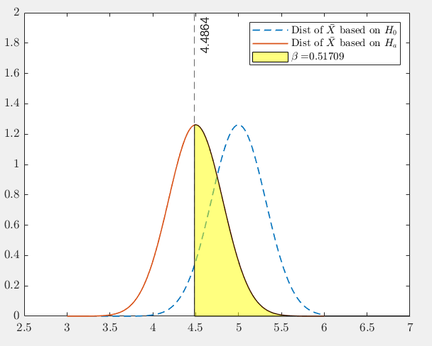
Figure 9.2: Probability of making Type II error

In Figure 9.2, we can see the \(\beta\) is quite large. The reason is that the value of \(\mu\) stated in the null hypothesis is so close to the true one (with the difference of only \(0.5\)), that the testing procedure can hardly tell the difference.

If the true population mean is \(\mu=4\), which is quite different from \(H_0: \mu=5\), then the probability of making type II error becomes smaller, as is seen in Figure 9.3 \[ \beta =P(\bar X > 4.4798 \mid \mu=4)\approx0.06. \]

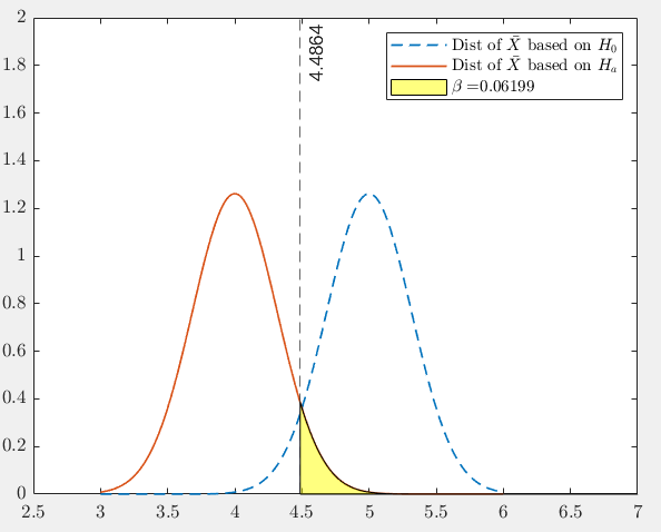
Figure 9.3: Probability of making Type II error

The value of \(\beta\) is depending on the difference between the true value of \(\mu\) and the one proposed in \(H_0\). The larger the difference is, the less likely that we will make type II error.

The difference of the true parameter and the value in \(H_0\) is called “effect size”;

Large effect size makes it easier for the testing procedure to spot the effect. (You may interpret the effect as the efficacy of the new drug compared with the placebo. If the new drug is very effective, the clinical trial procedure can easily tell the difference).

9.4.2 Power

The power of hypothesis procedure is defined by the probability of rejection when the null hypothesis is false, which is \[ P(rejection\mid H_0 \text{ is false})=1-P(acceptance\mid H_0 \text{ is false})=1-\beta. \] Intuitively, you can interpret the power as the possibility of proving the new research statement, which is formulated in the alternative hypothesis \(H_a\).

In practice, we often control the power by at least \(80\%\), which means the probability of making type II error is at most \(20\%\).

9.5 Summary of Tests on Population mean

Assumption: the population is normally distributed with population mean \(\mu\) and population standard deviation \(\sigma\) \[ X \sim N( \mu, \sigma). \]

9.5.1 Z-test

Use when the population standard deviation \(\sigma\) is known.

Tests	left-sided z-tests	right-sided z-tests	two-sided z-tests
Hypotheses	\(H_0: \mu=\mu_0\) vs \(H_a: \mu<\mu_0\)	\(H_0: \mu=\mu_0\) vs \(H_a: \mu>\mu_0\)	\(H_0: \mu=\mu_0\) vs \(H_a: \mu\ne\mu_0\)
Test statistics	\(Z=\frac{\bar X-\mu_0}{\sigma/\sqrt n}\)	\(Z=\frac{\bar X-\mu_0}{\sigma/\sqrt n}\)	\(Z=\frac{\bar X-\mu_0}{\sigma/\sqrt n}\)
Decision rule	Reject \(H_0\) if \(z< -z_\alpha\)	Reject \(H_0\) if \(z>z_\alpha\)	Reject \(H_0\) if \(z<-z_{\alpha/2}\) OR \(z>z_{\alpha/2}\)
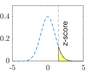
P-value	\(\Phi(z)\)	\(1-\Phi(z)\)	\(2(1-\Phi(|z|))\)
P-value (graphic)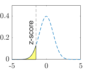

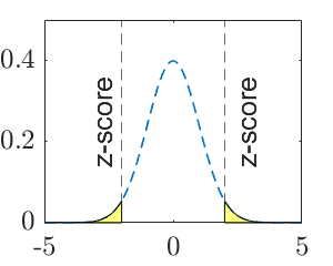Note: \(\mu_0\) is a specific number, such as \(15\). \(z\) is the observed test statistic and \(z_\alpha\) is the critical value for significance level \(\alpha\). The calculated value of test statistic is called z-score, which is an instance of the test statistic for a specific data set.

Table of Critical values for z-tests:

Level of Significance \(\alpha\)	Left-sided \(-z_{\alpha}\)	Right-sided \(z_{\alpha}\)	Two-sided \((\pm z_{\alpha/2})\)
0.01	\(-2.33\)	\(2.33\)	\(\pm2.575\)
0.05	\(-1.645\)	\(1.645\)	\(\pm1.96\)
0.1	\(-1.28\)	\(1.28\)	\(\pm1.645\)

9.5.2 T-test

Use when the population standard deviation \(\sigma\) is unknown and estimated by sample standard deviation \(S\).

Tests	left-sided t-tests	right-sided t-tests	two-sided t-tests
Hypotheses	\(H_0: \mu=\mu_0\) vs \(H_a: \mu<\mu_0\)	\(H_0: \mu=\mu_0\) vs \(H_a: \mu>\mu_0\)	\(H_0: \mu=\mu_0\) vs \(H_a: \mu\ne\mu_0\)
Test statistics	\(T=\frac{\bar X-\mu_0}{S/\sqrt n}\)	\(T=\frac{\bar X-\mu_0}{S/\sqrt n}\)	\(T=\frac{\bar X-\mu_0}{S/\sqrt n}\)
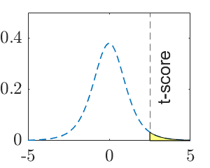
Decision rule	Reject \(H_0\) if \(t< -t_{\alpha, n-1}\)	Reject \(H_0\) if \(t>t_{\alpha, n-1}\)	Reject \(H_0\) if \(t<-t_{\alpha/2, n-1}\) OR \(t>t_{\alpha/2, n-1}\)
P-value (graphic)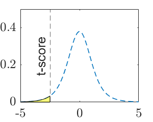

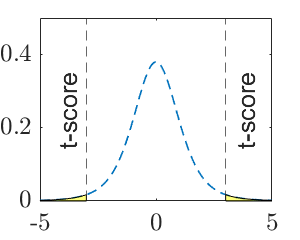Note: \(\mu_0\) is a specific number, such as \(15\). \(t\) is the observed test statistic and \(t_\alpha\) is the critical value for significance level \(\alpha\). The calculated value of test statistic is called t-score, which is an instance of the test statistic for a specific data set.

9.5.3 Large sample-test

Use when the population standard deviation \(\sigma\) is unknown and estimated by sample standard deviation \(S\) AND the sample size \(n\) is large.

Tests	left-sided z-tests	right-sided z-tests	two-sided z-tests
Hypotheses	\(H_0: \mu=\mu_0\) vs \(H_a: \mu<\mu_0\)	\(H_0: \mu=\mu_0\) vs \(H_a: \mu>\mu_0\)	\(H_0: \mu=\mu_0\) vs \(H_a: \mu\ne\mu_0\)
Test statistics	\(Z=\frac{\bar X-\mu_0}{S/\sqrt n}\)	\(Z=\frac{\bar X-\mu_0}{S/\sqrt n}\)	\(Z=\frac{\bar X-\mu_0}{S/\sqrt n}\)
Decision rule	Reject \(H_0\) if \(z< -z_\alpha\)	Reject \(H_0\) if \(z>z_\alpha\)	Reject \(H_0\) if \(z<-z_{\alpha/2}\) OR \(z>z_{\alpha/2}\)
P-value	\(\Phi(z)\)	\(1-\Phi(z)\)	\(2(1-\Phi(|z|))\)
P-value (graphic)